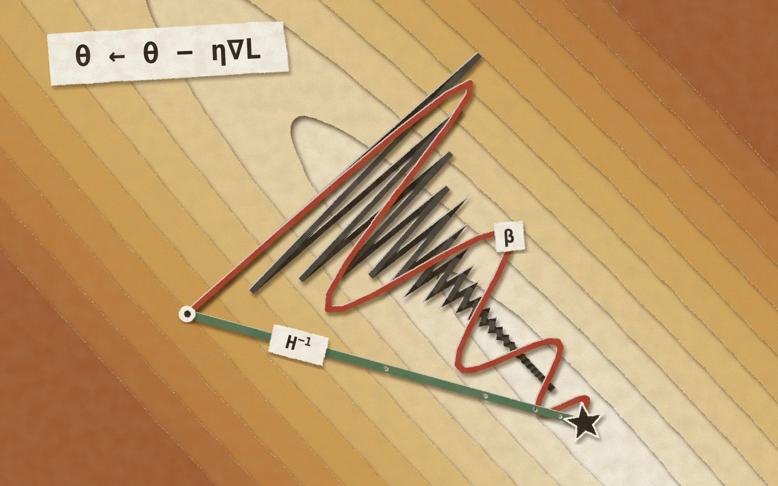
Open a PyTorch training script, and the loop almost always contains these two lines:
loss.backward()
optimizer.step()
backward() works out which direction each parameter should change in, and step() actually makes the change. This article is about the few lines inside step().
The directions have already been computed, so why not just follow them? It doesn't sound like there's much to say. Yet “how to take this one step” alone has sprouted a whole family, from SGD, Momentum, AdaGrad, Adam, and AdamW all the way to Lion and Muon. Almost every new method appeared because the one before it walked poorly on some kind of terrain.
We'll start from the very basics, with one straight line and twelve parcels. First we draw the “gradient”, then walk it through a long, narrow valley, random noise, cliffs, and saddle points, and see which gap each method fills in the one before it.
Before we set off, take a look at the whole route. Each row is a method, followed by the gap it fills:
Basics
- BGDThe starting point: every step reads all the data.
- SGD · MBGDReading all the data per step is too slow → sample one item or a small batch.
- SGDMZigzags and noise → accumulate a velocity.
- NAGMomentum overshoots → take the gradient at the look-ahead point.
One step size per parameter
- AdaGradOne learning rate for every parameter → scale each by its accumulated gradients.
- RMSProp · AdaDeltaAdaGrad's rate only ever shrinks → a moving average that can forget.
- Adam · NadamCombine momentum with per-parameter steps, and correct the zero-start bias.
Fixing Adam
- AMSGradAdam can converge to the wrong point → never let v shrink.
- AdamWInside Adam, L2 gets divided by √v̂ → decouple weight decay.
- Warmup · Cosine · SGDR · RAdam · Schedule-FreeHow should the rate change, and why does Adam need warmup? → schedules, a rectified variance, or no schedule at all.
Scale and geometry
- LARS · LAMBHuge batches: layers differ in ‖w‖/‖g‖ → a trust ratio per layer.
- Adafactor · GaLoreOptimizer state eats memory → factor it, or keep it in a low-rank subspace.
- SAMA low loss in a narrow valley → compare the worst loss within ρ.
- Shampoo · SOAP · SophiaDiagonal scaling can't fix a tilted valley → matrix preconditioners, or curvature with clipping.
- LionLess state and computation → keep only the sign.
- MuonWeights are matrices, not long lists → orthogonalize the whole update.
Every animation in this article is computed live in your browser, and each step uses exactly the formula written in the text. Press pause, and you can drag the slider to go through it one step at a time.
Start with a straight line
Suppose you run a small online shop and have just shipped 12 parcels. They weigh between 0.5 and 1.5 kg, and their shipping fees range from NT$92 to NT$150.
The fee looks roughly like “base fee + a surcharge per kg”, which we can write as a straight line:
is the weight (kg), is the predicted shipping fee (in units of NT$100), is how much each kilogram adds, and is the base fee. From these 12 records, we want to find the best-fitting and .
Start with an arbitrary guess, NT$210 per kg plus a base fee of NT$20, that is, , . This line is too steep. It overestimates all 12 parcels, overcharging the lightest by NT$32 and the heaviest by NT$185.
How do we measure “how bad the guess is”? Square each parcel's error, then take the average:
Squaring keeps positive and negative errors from canceling each other out, and it also penalizes parcels that are far off more heavily. The in front is only there to cancel the 2 that the square brings down when we take the derivative in a moment.
This is called the loss function. Plugging in our guess gives .
Next comes the most important idea in the whole article.
Every pair is a straight line, and each one has a loss value. Put on the horizontal axis and on the vertical axis, mark the loss at every point of the plane, and you get a terrain map. The lower the loss, the lower the ground. Finding the best line means finding the lowest point on this terrain.
The rings on the map are contour lines. Every point on the same ring has the same loss, and the closer you get to the star in the middle, the lower the loss. The star sits at , , that is, NT$59 per kg plus a base fee of NT$61, where .
Notice the shape of this terrain. It's a tilted valley, long and narrow. This shape will follow us through the whole article, and many of the methods later on are trying to deal with it.
Slope and gradient
Standing at some point on the terrain, how do you know which way is downhill?
Let's simplify first. Fix at its best value and move only , and the terrain reduces to a single curve. The slope of the tangent at any point on the curve is the derivative :
A positive slope means the loss grows as grows, so downhill is to the left; a negative slope means downhill is to the right; a slope of 0 means you've reached the bottom. Moving against the slope means moving downhill.
When both parameters can move, each has its own partial derivative, the slope when “only it moves and everything else stays put”. For our loss function:
Stack them into a vector, and that's the gradient:
These two expressions aren't hard to read. Take each parcel's error, multiply it by this parameter's influence on that parcel, and average. has an influence of 1 on every parcel; 's influence is the parcel's weight , so the heavier the parcel, the more say it has about .
At the starting point , all 12 parcels are overestimated, and the calculation gives . Both components are positive, which means that increasing either or would make the loss larger.
The figure shows two properties of the gradient:
- It points in the direction of steepest ascent, so is the direction of steepest descent.
- It is perpendicular to the contour line through that point.
Why? Near a point , take a small step , and the loss changes by roughly
This is a first-order Taylor expansion. The dot product can be written as , where is the angle between the gradient and the step. For a fixed step length, the loss drops the most when , that is, when you walk opposite to the gradient. Walking along a contour line leaves the loss unchanged, so and the angle is ; that's why the gradient is perpendicular to the contour.
BGD: follow the negative gradient
Once you know which way is downhill, the rest is simple. Take a small step toward , then repeat:
(eta) is the learning rate, which sets how far each step goes. This is gradient descent. Because every step computes the gradient from all 12 parcels, it's also called batch gradient descent (BGD).
The idea is older than computers. The earliest written record we can find is a three-page note by Cauchy from the session of the French Academy of Sciences on October 18, 1847, “Méthode générale pour la résolution des systèmes d'équations simultanées”, printed in Comptes Rendus, volume 25, pages 536 to 538. He wanted to solve the simultaneous equations that determine the orbit of a celestial body. His approach was to square each equation and add them up, then keep shrinking this sum by moving in the direction of the negative partial derivatives. There was no fixed learning rate yet. Cauchy gave several ways to choose the step, one of which was to keep searching along this direction and stop only at the point where the function is smallest.
With , the first step is:
The loss drops from 0.71 to 0.040, losing more than 90% in a single step.
A beautiful first step. What comes next?
Once the point drops into the valley, it crawls slowly along the valley floor. In the parcel plot, the line has long since settled close to the data, and the hundred-odd steps that follow are only fine-tuning; it takes until step 168 to get within 0.03 of the minimum.
Why so slow? Would turning up a little help?
Learning rate: how far to step
Let's go back to the simplest case first, a one-dimensional bowl . is the bowl's curvature, that is, its second derivative; the larger it is, the steeper the bowl. The gradient is , so each step is:
Every step multiplies by once more.
In the figure, , and the four runs differ only in :
- : each step shrinks it by only 10%, a slow crawl.
- : each step leaves only 10%, so it reaches the bottom quickly.
- : , so every step jumps to the other side, but lands closer each time; it converges while swinging back and forth.
- : , so every step jumps to the other side and lands even farther out; the swings keep growing, and it diverges.
So the condition for convergence is , that is, . The steeper the bowl, the smaller the learning rate has to be.
A long, narrow valley
Our terrain is two-dimensional, and the trouble is that it has two curvatures.
Cut across the valley and the terrain is steep; follow the valley floor and it's very flat. In linear-algebra terms, these are the two eigenvalues of the loss's matrix of second derivatives (the Hessian), which in this example are 2.05 and 0.045, a factor of 46 apart. This ratio is called the condition number, written .
The same has to take care of both directions at once. To avoid diverging in the steep direction, must be smaller than ; but then in the flat direction, each step can shrink the remaining distance by at most , so it takes at least several dozen steps. Make a little larger and the steep direction bounces back and forth; make a little smaller and the flat direction barely moves.
With , the point bounces back and forth in the steep direction, tracing a zigzag while it slowly advances along the valley floor, and doesn't arrive until step 93.
Why is this valley tilted? The valley floor runs roughly along , that is, up by 1 and down by 1. For a 1 kg parcel, the predicted fee doesn't change at all. The average weight of these 12 parcels happens to be exactly 1 kg, so adjusting along this direction barely affects the predictions overall, and the loss hardly changes. The slope and the intercept cancel each other out, and that forms a tilted valley.
Click “minus the mean” on the figure to subtract 1 kg from every parcel's weight, and the model becomes . It can draw exactly the same lines, but and the new intercept no longer pull against each other. The valley straightens out, the condition number drops to 10.9, and it arrives at step 46. Then divide by the standard deviation as well, which is “standardization”, and the slope becomes a new too. The curvatures in the two directions become equal, the valley turns into a round bowl with a condition number of 1, and it arrives in two steps.
This is why inputs are often standardized before training. But a deep network easily has hundreds of millions of parameters, and the inputs to every layer keep changing, so we have no way of reshaping the terrain by hand one piece at a time.
The methods that follow attack the problem from roughly three directions:
- Remember the direction you just came from, so the back-and-forth bouncing cancels out (momentum).
- Give each parameter its own step size (AdaGrad, RMSProp, Adam).
- Estimate the shape of the terrain, or measure a step with a different ruler (Newton's method, Shampoo, Muon).
Hitting a cliff
Too large a learning rate makes it diverge. But sometimes, even with a modest learning rate, a single step can fling you out.
This terrain is a gentle slope followed by a steep wall. The point follows the slope to the wall, and one step happens to land on the wall's face. The gradient on the wall is huge, and the next step bounces the point straight to , out of the frame. It spends nearly ten steps climbing back to the wall, then lands on the face again and gets bounced out again; in 40 steps it's thrown out three times, twice right out of the frame.
Real RNNs have walls like this too. In 2013, while analyzing why RNNs are hard to train, Pascanu, Mikolov, and Bengio put forward a hypothesis. In the directions where gradients explode, the curvature is usually large as well, so the loss surface forms a steep wall; step onto it, and you're flung out of the valley you were in. In On the difficulty of training recurrent neural networks, they drew such a wall using an RNN with a single hidden unit.
The fix is straightforward. When the gradient is too large, scale it down. The most common version is clipping by norm:
If the gradient's length exceeds , it gets scaled down to with its direction unchanged. The “clip to 1” panel caps the gradient's size at 1, and the point keeps making small moves back and forth by the wall instead of flying off. In PyTorch, this is torch.nn.utils.clip_grad_norm_.
What should be? Pascanu et al. suggest first watching the average gradient norm over a stretch of training; anything from half of it to ten times it still converges, though the speed is affected.
SGD and MBGD: a few samples at a time
BGD has to go through all of the data for every single step. With 12 parcels, that's no problem; switch to ImageNet's 1.28 million training images, and every step means running all 1.28 million images through a forward and a backward pass first.
Stochastic gradient descent (SGD) draws just one random sample per step and uses its gradient in place of the gradient over all the data:
is the loss of sample on its own, and is the sample drawn at step .
With only one sample, the gradient is of course inaccurate. But if every sample is equally likely to be drawn, its expected value is exactly the full gradient:
On average the direction is right; each step just carries some noise.
The compromise is to draw a small batch each time, say 4 samples, and average their gradients. This is called mini-batch gradient descent (MBGD). The larger the batch, the smaller the noise; the variance of the gradient is roughly inversely proportional to the batch size.
All three routes use the same . BGD is the smoothest; MBGD wobbles slightly all the way; SGD shakes the most, and the circled parcel in the parcel plot is the one it drew for this step.
But look at how much data each one has read. All three get within 0.03 of the minimum at around step 170. BGD reads 12 samples per step and has read 2,016 by the time it arrives; MBGD has read 676; SGD only 178. Measured by the amount of data read, the shakiest route is the cheapest.
The learning rate has to shrink
SGD has a problem that BGD doesn't. At the minimum, the full gradient is 0, but each parcel's own gradient isn't. The 12 parcels can't all lie exactly on the same line, so every one of them is still pulling the parameters toward itself. Whichever parcel gets drawn, the parameters drift a little its way.
This figure starts right at the minimum and looks at one sample at a time. With a fixed learning rate, the parameters keep circling around the minimum, and over the last 50 steps their average distance from it is 0.042; when the learning rate shrinks with the step count as , the circling narrows along with it, and the average distance drops to 0.015.
So how should the learning rate shrink? Shrink it too fast and you stop before you get there; too slowly and the noise never goes away.
Finding the minimum means finding the point where , that is, finding the root of an equation. Robbins and Monro's 1951 “A Stochastic Approximation Method” studied exactly this kind of problem, except that every observation they could make was noisy. Later authors distilled their step-size conditions into two:
The first makes the total distance long enough to get there however far away you start; the second keeps the total accumulated noise finite, so you can come to a stop in the end. satisfies both, and the decay in the figure above belongs to this family.
Noise has its uses
SGD's noise isn't all bad.
This terrain is . The origin is a saddle point. Along the direction it's a valley floor, along the direction it's a hilltop, and the gradient there is 0. The two real valley floors are at .
GD starts from . Its gradient in the direction is 0 from the start and stays 0 forever, so it slides all the way into the saddle point and stops there. Add a tiny bit of noise (a standard deviation of just 0.0001), and when the point nears the saddle it gets gently nudged off the ridge, dropping into the valley floor at by step 64.
In a two-dimensional figure, a saddle point looks like a special case. Dauphin et al.'s 2014 “Identifying and attacking the saddle point problem in high-dimensional non-convex optimization” argues that the higher the dimension, the more saddle points there are relative to local minima, and that slow training is often due to getting stuck on the flat plateaus near saddle points, rather than falling into bad local minima.
Noise can help you escape, but in theory this comes with conditions. Ge et al. proved in 2015 that if every saddle point has a clear downhill direction (negative curvature), the function is smooth enough, and the noise has variance in every direction, then noisy SGD escapes saddle points within a polynomial number of steps. Our example starts right on top of the ridge, a deliberately chosen worst case; from a random starting point, GD almost never stops exactly on a saddle point, though it may move very slowly across a flat plateau.
SGDM: remember where you were going
Back to the long, narrow valley. The problem with the zigzag is that in the direction across the valley, the gradient flips sign at every step, pushing toward one side of the valley this step and back to the other side the next. In the direction along the valley floor, the gradient is small, but it always points the same way.
If each step looked not only at the current gradient but also at the gradients of the previous few steps, the parts that flip back and forth would cancel out, and the part that keeps pointing the same way would build up.
Exponential moving average
The most common way to “look at the previous few steps” is the exponential moving average (EMA):
The new average is the old average times , plus the new gradient times . With , the new gradient gets a 10% share; a gradient from ten steps ago still keeps of its influence, and the older a gradient is, the fainter it gets. There's no need to store past gradients one by one; a single number is enough.
We split the gradients from GD's path through the valley into two components, across the valley and along it. The across component is about 1.7 at the first step and alternates in sign after that, and the EMA quickly flattens it to near 0; the along-the-floor component is only about 0.06, but its direction never changes, and the EMA holds on to it steadily.
Momentum
Use this average to update the parameters, and you have momentum. SGD with momentum is often abbreviated SGDM:
This drops the factor, so it's times the EMA above. When the gradient keeps pointing the same way, builds up to , which is 10 times for . The small gradient that couldn't get anywhere in the flat direction gets amplified this way.
The metaphor comes from physics. is like the velocity of a ball, the gradient is the push the slope gives it, and decides how much of the velocity is kept at each step.
This idea also predates deep learning by a long way. In 1964, Polyak wrote it as
that is, on top of the gradient step, add “the previous displacement” times . Eliminate from the two lines above, and you get exactly the same expression, with being . Polyak himself called it the heavy ball method, viewing it as a discrete version of an object moving in a potential field, and recommended taking between 0.8 and 0.99 in most cases.
He also worked out how much it speeds things up. On a quadratic with condition number , the number of steps GD needs is roughly proportional to , while the heavy ball method needs a number proportional only to . Our valley has , so . But this result holds only on quadratics, or near a minimum where the function looks enough like one. In 2016, Lessard et al. constructed a one-dimensional function with condition number 25 on which the heavy ball method, run with the optimal parameters for quadratics, falls into oscillations that never die down.
With the same , GD doesn't arrive until step 93; add momentum with , and it arrives at step 19.
Look closely at the momentum route. At first it's no better behaved; in fact, it swings widely across the valley several times. What momentum cancels is the kind of bouncing that flips sign every step; the velocity the ball has already built up still takes several steps to come to a stop.
What happens if is too large?
All three panels use . remembers too little and helps only a bit, failing to arrive within 200 steps; arrives at step 51; has almost no friction, so the ball circles around and around near the valley floor and doesn't settle within 200 steps either.
NAG: look before you step
Momentum is slow to react. Near the bottom, the ball overshoots with the velocity it has built up, and only turns back after the gradient has pushed the other way for several steps.
Nesterov momentum (Nesterov Accelerated Gradient, NAG) changes just one thing. Since this step will move along the velocity anyway, go there first, check the slope there, and then decide how to correct:
The only difference is where the gradient is computed. Momentum computes it at the current position; NAG computes it at the look-ahead point, “where one step at the current velocity would take you”. If the ground ahead has already started to rise, NAG feels it a step early and taps the brakes a little in advance.
The hollow circles are NAG's look-ahead points. With the same and , momentum arrives at step 37 and NAG at step 22.
Why does it work especially well in a valley? Sutskever et al. showed in 2013 that on a quadratic, NAG amounts to using a different momentum in each eigendirection, where is the curvature in that direction. The larger the curvature, the smaller the momentum. Plugging in this figure's settings, the direction across the valley has , leaving an effective momentum of only , with almost no drive left; the direction along the floor has and keeps 0.78. Directions prone to bouncing get damped, and directions that need speeding up still speed up.
The method comes from Nesterov's 1983 paper, where it was originally a theoretical result in convex optimization, guaranteeing that the error decreases at a rate of . The “compute the gradient at the look-ahead point” formulation is a rewrite by Sutskever, Martens, Dahl, and Hinton in “On the importance of initialization and momentum in deep learning”. They had momentum rise slowly from a small value to 0.99 or even 0.999, paired it with carefully designed initialization, and got SGD with momentum to match the more complex second-order methods of the time on deep autoencoders.
AdaGrad: every parameter goes its own way
So far, all parameters have shared the same .
For many problems, that doesn't make sense. The AdaGrad authors, Duchi, Hazan, and Singer, use text data as their example. Common words show up in every sample, so their parameters are updated all the time; rare words appear only once in a while, but when they do, they're often highly predictive. The same learning rate may be too large for the former and too small for the latter.
AdaGrad has each parameter keep the sum of all its past squared gradients, and divides by its square root:
The squaring, square root, and division here are all done separately for each parameter. is a very small number that prevents division by zero.
A parameter whose gradients are always large sees grow fast, so its steps get smaller; a parameter that rarely gets updated has a small , so it can take a big step as soon as a gradient comes along. The first step is even more interesting. , so every parameter's first step is , no matter how large the gradient itself is.
With , the first step moves and by exactly 0.5 each. After that, the effective learning rates of the two parameters sit at about 0.39 and 0.45 and practically never move again. 97% of comes from the first five steps. At the start, you're far from the minimum and the gradients are large, so each square adds a big chunk; later the gradients keep shrinking, and adding more of them barely makes a difference. This run doesn't get within 0.03 until step 203, slower than BGD's 168 steps.
only ever grows, so each parameter's effective learning rate only ever shrinks, and it's set mainly by those first few steps. On convex problems, this is exactly the mechanism that makes it converge; but training a deep network takes hundreds of thousands of steps over terrain that keeps changing, and the learning rate often becomes too small to move before it gets anywhere good.
RMSProp and AdaDelta: learning to forget
Since the trouble comes from “adding up every past gradient”, just remember the recent ones.
Replace AdaGrad's running sum with an exponential moving average, and you get RMSProp:
is usually 0.9. The here tracks the average of the squared gradients, which is a different thing from the velocity in the momentum section. Large gradients from long ago are gradually forgotten, so the effective learning rate can shrink and can also grow back.
RMSProp has an unusual history. It has no paper. It comes from the slides for Lecture 6, section 5 (Lecture 6e) of the Coursera course “Neural Networks for Machine Learning” that Hinton taught in 2012. The slide shows exactly , then divides the gradient by its square root, and notes that this is unpublished work by Tijmen Tieleman. Later papers that cited it could only cite these lecture slides.
The terrain in this figure starts with a steep stretch of slope 1, followed by a long, gentle stretch with a slope of only 0.1, and the bottom is at . Both start from ; AdaGrad uses , and RMSProp uses , .
On the steep stretch, both denominators get inflated by the large gradients. Once on the gentle stretch, AdaGrad's still remembers every step on the steep part, and its step size drops to about 0.01; RMSProp forgets quickly, its denominator shrinks along with the gradient, and its step size comes back to about 0.1. By step 100, AdaGrad has only reached , while RMSProp is already at 5.1; RMSProp reaches the bottom around step 150, while AdaGrad, by step 240, has only made it to 3.45. The one given the larger learning rate turns out to be the slower one.
That same year, Zeiler's AdaDelta used the same moving average and thought one step further. He noticed that the updates of SGD and AdaGrad have mismatched units. A gradient's units are “loss ÷ parameter”, so using it to update a parameter gets the units wrong; only after also dividing by a second derivative (we'll see this again with Newton's method) do the units come back to “parameter”. AdaDelta doesn't actually compute any second derivatives. Instead, it replaces the in the numerator with the root mean square of “past updates”:
Once the units of the numerator and denominator cancel, the update has the same units as the parameter, and you don't even need to set a learning rate.
Adam: putting the two together
At this point, we have two tools in hand. Momentum uses a moving average of the gradient to deal with directions that keep flip-flopping; RMSProp uses a moving average of the squared gradient to adjust the step size for each parameter.
Adam, proposed by Kingma and Ba in 2014, puts the two together:
is the first-moment estimate of the gradient, that is, its mean; is the second-moment estimate, that is, the mean of its square. In the Adam paper, the learning rate is written , playing the same role as earlier. The paper's defaults are , , , , and these numbers are still PyTorch's defaults today.
We've seen the first two lines before; the third is new.
Bias correction
Both and start from 0. At the first step, , only a tenth of the true gradient; , only a thousandth. Both estimates are dragged down by the zero they started from.
Expand and assume the gradient's expected value stays at , and you can work out that . So dividing by corrects the bias; the same goes for .
Why is the correction a must? The two estimates are biased by different amounts. drags down much more than , so without correction the denominator is too small and the steps are too big.
Suppose the gradient is a constant 1. The corrected is 1 from the very first step, so the step size is exactly . Without correction, the first step is times as large, shoots up to 6.6 times around step 12, and is still 1.26 times at step 1,000. In their variational autoencoder experiments, Kingma and Ba saw that the closer is to 1, the more unstable training without bias correction is at the start.
Each step is about
After correction, falls roughly around . Multiply the whole loss by 100, and the gradient is multiplied by 100 too; and scale up together, and apart from the tiny , the update barely changes. Each parameter moves about per step, regardless of how large the gradient itself is.
This is the main reason Adam is so easy to use. SGD's learning rate has to be tuned to the scale of the gradient; Adam's is closer to “how much you want the parameters to move per step”, and when you switch to a different model, the default often still works.
Four methods in the same valley, each with its learning rate tuned to a value that works well here; the numbers are the steps at which each first gets within 0.03 of the minimum. All four use the gradient over all 12 parcels, so the first two are GD without sampling and GD with momentum. GD () arrives at step 93; momentum (, ) at step 47; RMSProp () at step 130; Adam () at step 87.
Adam isn't much faster. We'll save the reason for the section on “making the valley round”; it has to do with the valley being tilted.
Adam can also use Nesterov momentum. In 2016, Dozat worked NAG's “look first” into Adam and called it Nadam. NAG first takes a step along the momentum and then measures the gradient; Nadam doesn't compute an extra gradient, but uses “the next step's momentum” directly in the update, plus this step's gradient. The NAdamW baseline later used by AlgoPerf (a public benchmark that compares how fast training algorithms are; more on it in the “Which one is fastest?” section) is Nadam plus the AdamW weight decay from the next section.
Adam gets things wrong too
Adam quickly became the default choice. But over the next few years, people pointed out its problems one after another.
Forgetting the big gradients that matter
Reddi, Kale, and Kumar constructed a tiny example. The parameter is restricted to , and every three steps form one cycle; the loss is at the first step and at the other two. With , the total gradient over one cycle is , so should be pushed toward .
Adam's denominator is what goes wrong here. As soon as the rare large gradient 3 appears, jumps up right away, and this step's is squashed to about 1.05; for the next two steps the gradient is only , quickly shrinks again, and these two steps are inflated to and . Over one cycle, measured in units of , it ends up 0.68 further in the wrong direction.
Both start from , with a learning rate of . Adam gets pushed back to every three steps and stays stuck at the wrong end; AMSGrad reaches about by step 100 and by step 300.
Here and , settings the paper chose for the proof. The root cause is that Adam's effective learning rate can grow. Once the recent gradients are small, the large gradients of the past are forgotten.
Their fix, AMSGrad, changes only one thing. The denominator uses the largest seen so far:
From then on, the effective learning rate can only shrink, never grow. In the example above, all three steps use the same , and the net effect over one cycle becomes a move of 0.35 in the right direction.
Worse generalization?
Another challenge came from Wilson et al.'s 2017 “The Marginal Value of Adaptive Gradient Methods in Machine Learning”. They constructed a linear classification problem on which the solution SGD finds has a test error of 0, while the solutions found by AdaGrad, RMSProp, and Adam put every new sample into the same class.
On CIFAR-10, tuning only the learning rate and its decay scheme, they got a test error of 7.65% for SGD, 9.60% for RMSProp, and 9.78% for Adam. The training loss went down fast, but the test results were worse. This paper kept a fair amount of computer vision research on SGD with momentum.
Two years later, Choi et al. reran the experiments with Wilson et al.'s public code, tuning momentum and as well, and the test errors of the four methods came out nearly the same. How large the gap is depends to a great extent on which hyperparameters get tuned.
Weight decay gets shrunk
The third problem is the hardest to spot, and it has had the biggest impact.
Weight decay pulls the parameters a little toward 0 at every step, keeping them from growing too large. In SGD, it's equivalent to L2 regularization. Add to the loss, and the gradient gains an extra term , whose effect is to shrink the parameters a little each step.
So early Adam implementations simply added to the gradient. But inside Adam, this term also gets divided by . For a parameter whose gradients are always large, is large, and the decay is shrunk to very little; in Loshchilov and Hutter's words, weights with larger past gradients get regularized less.
Their fix is to take the decay out so it doesn't go through Adam's denominator:
This is AdamW. In the formula, is the learning rate, and is the multiplier the learning-rate schedule gives at step , which is 1 when the learning rate is fixed.
Both weights start from 1, their gradients are pure noise, and the sizes of the two noises differ by a factor of a thousand. , . In the version that adds L2 to the gradient, , with the large gradients, is hardly decayed at all and is still at 0.96 after 500 steps; , with the small gradients, is instead pulled down by about 0.002 per step and falls to 0.28 by step 500. AdamW treats the two weights the same, multiplying each by 0.996 at every step, and by step 500 both are down to around 0.13.
In the CIFAR-10 experiments, the good results for Adam with L2 lie along a diagonal line in learning rate and , so tuning one means retuning the other; AdamW's good region runs roughly parallel to the two axes, so the two hyperparameters can be tuned separately, and its best result also caught up with SGD. Today, AdamW is practically the default for training Transformers and large language models.
Learning-rate schedules
We said earlier that SGD's learning rate has to shrink gradually. But shrink how?
From steps to cosine
The earliest and most common is the step schedule, which divides by 10 every so often. The classic recipe for training ResNet-50 is 90 epochs (one complete pass over the whole training set is called an epoch), dividing by 10 at epochs 30, 60, and 80. Its drawback is that you only get a good model after the last division, and you have to decide for yourself when to divide.
In 2016, SGDR switched to a cosine curve that decreases smoothly from the maximum to the minimum:
is how long the current cycle has been running, and is the length of this cycle. At the end of a cycle, the learning rate jumps straight back to the maximum and the next cycle begins, which is called a warm restart; the next cycle's length can be multiplied by , so the cycles get longer and longer. It was proposed by none other than Loshchilov and Hutter, who later wrote AdamW.
The figure shows five schedules, with the cursor moving in sync. The SGDR panel uses and , restarting at epochs 10, 30, and 70.
Restarts never really caught on. In SGDR's own experiments, the best single model for WRN-28-10 on CIFAR-10, at 3.86%, came from a cosine with no restarts at all, just one cycle. The training setups of GPT-3 and LLaMA later used a single-cycle cosine as well. What stuck was the smooth curve, at the cost of having to know the total number of steps in advance once again; the experiments in Chinchilla (DeepMind's paper on how model size and the amount of training data should be matched) found that if the cosine cycle is longer than the actual number of training steps by 25% or more, the results get noticeably worse.
Without fixing the finish line in advance
A cosine schedule needs to know the total training length up front. But when training large language models, people often decide halfway through whether to train a bit longer.
In 2024, MiniCPM used a three-phase schedule called WSD (Warmup-Stable-Decay). It starts with warmup (covered in the next section), then holds the learning rate constant for a long time, and lowers it only over roughly the last tenth of training. Any checkpoint (a model saved partway through training) from before the decay can be picked up and trained further at any time.
In 2024, Defazio et al. went even further and did away with the schedule altogether. Schedule-Free maintains three sets of parameters at once:
Here , , and are three sets of parameters, unrelated to the parcel weight . is plain SGD with a fixed step size ; is the average of all the 's, and it's also the model you end up using; the gradient is computed at , which sits between the two. Averaging the past 's works like a linear decay whose endpoint keeps moving along with the current step count.
Each step draws 4 parcels, with and . For the first hundred-odd steps, clearly lags behind , because it gives every equal weight, including the earliest 's, far from the minimum; the longer it runs, the steadier gets.
In the 2024 AlgoPerf training-algorithm competition, Schedule-Free AdamW won the track that forbids external hyperparameter tuning, averaging about 8% faster than the baseline, and it was also the only submission in that track to beat the baseline. It still needs warmup, though. Most of the paper's experiments set warmup to 5% of total training, so the total length still comes in through the warmup.
Warmup
These days, almost every training config specifies that over the first few thousand steps, the learning rate should climb slowly from something very small. This is called warmup. Why can't you just use a large learning rate from the start?
Linear scaling and warmup
Warmup was first written up as a recipe in Goyal et al.'s 2017 “Accurate, Large Minibatch SGD: Training ImageNet in 1 Hour”. They wanted to grow the batch from 256 to 8,192 and train ResNet-50 in one hour on 256 GPUs.
The first rule is linear scaling. When the batch grows -fold, the learning rate grows -fold too, so the learning rate for batch 8,192 is 3.2. But the network changes very fast at the start of training, and using such a large learning rate right away wrecks the model. So over the first 5 epochs, the learning rate rises linearly from the original 0.1 to 3.2.
Without warmup, the top-1 error (the fraction of images where the first guess is wrong) is 24.84%; warming up with a fixed small learning rate is actually worse, at 25.88%; gradual warmup gets 23.74%, catching up with the 23.60% of batch 256. Up to a batch of 8,192, the error barely changes; it starts getting worse at 16k, reaching 27.55% at 32k and 33.96% at 64k.
Why Adam needs warmup too
Adam's step size is roughly , so in principle it shouldn't be afraid of large gradients. Why, then, does Adam without warmup still often break right at the start when training Transformers?
RAdam's authors, Liu et al., offered an explanation in 2019. At the start of training, has seen only a few gradients, so its estimate of “how large the gradient is” is very unreliable. The first step is even more extreme. , so the adaptive learning rate is estimated from a single sample, and its variance actually diverges.
The figure shows 2,000 simulations, with gradients drawn from a standard normal distribution and . In the simulations, 90% of the values of at step 1 fall between 0.50 and 14.4, a spread of nearly thirty times; by step 10, they've already narrowed to between 0.73 and 1.6.
RAdam estimates how large this variance is and multiplies by a rectification term , skipping the adaptive learning rate altogether in the first few steps, while the variance is too large. With , the first 4 steps use momentum only, and after that climbs slowly from very small to 1, which works like a built-in warmup.
In October of the same year, Ma and Yarats pointed out that depends only on the step count and on , not on the data. So RAdam is roughly a fixed-length warmup, and their rule of thumb is steps, which comes to 2,000 steps for . Comparing the two with ResNet-50 on ImageNet, they found that a linear warmup of exactly this length comes within half a percentage point of RAdam.
When batches get bigger: LARS and LAMB
Goyal et al.'s recipe is very stable up to batch 8,192, but beyond that it can't hold up. The error rate is 24.79% at 16k, 27.55% at 32k, and 33.96% at 64k. What goes wrong as the batch keeps growing?
One explanation is that large batches find sharper minima. Keskar et al. observed in 2017 that models trained with a batch of 10% of the training set end up in sharper minima and have lower test accuracy. This explanation was later challenged. Dinh et al. proved that the sharpness of a ReLU network can be inflated arbitrarily without changing the function it computes; Hoffer et al. found that once the learning rate is scaled up with the square root of the batch size and the number of training steps is increased to compensate, the gap disappears.
The other problem is more direct. LARS's authors, You, Gitman, and Ginsburg, measured the weight norm and gradient norm of each layer of AlexNet-BN at the first step. The ratio of the two, , is 5.76 in the first convolutional layer and 1,345 in the first fully connected layer, more than two hundred times apart.
Under the same global learning rate, the relative change per step in the first convolutional layer is 234 times that of the fully connected layer. Once the learning rate passes a certain point, the first layer's update becomes larger than its weights, and training falls apart; yet for the fully connected layer, that learning rate is still tiny.
LARS computes a learning rate of its own for each layer, making the update proportional to the size of that layer's weights:
is a small trust coefficient, which the paper writes as and sets to 0.001; we use a different letter here so it isn't confused with the learning rate. This way every layer's relative change is equally large, and the most sensitive layer no longer holds the rest back. For AlexNet at batch 8k, without LARS and with warmup alone, the learning rate can't be scaled up no matter how it's tuned, and the best top-1 accuracy is 44.8%; with LARS it's back to 58.2%, close to the 58.7% of batch 512.
LAMB applies the same layer-wise scaling to Adam. It first computes this layer's update the Adam way, adds the weight decay , and then rescales the length of the whole update to be proportional to the length of this layer's weights:
is the weight of layer , and is a function that keeps the weight norm between a lower and an upper bound. In 2019, You et al. used it to cut BERT-Large pre-training from 81.4 hours on 16 TPUv3 chips to 76 minutes on 1,024 TPUv3 chips; the batch was 64k in the first phase and 32k in the second.
The story has a sequel. In 2021, Nado et al. retuned Adam and fixed two problems in BERT's open-source code, the missing bias correction and a cliff in the learning-rate schedule; with the same batch size and number of steps, Adam matched LAMB or even did slightly better. Well-tuned Nesterov momentum also matched LARS on the ResNet-50 setup of MLPerf (an industry benchmark for training speed).
Finding a flat valley floor: SAM
Back to Keskar et al.'s observation. Are sharp minima really worse?
All of the methods so far answer “how to get to the valley floor faster”. In 2020, Foret et al. asked a different question. Which valley floor is better?
Picture two valleys, one deep and narrow, the other shallow and wide. On the training loss, the narrow one is lower; but test data always differs a bit from training data, and when the parameters shift slightly, the narrow valley's loss shoots up while the wide valley's barely changes.
SAM (Sharpness-Aware Minimization) changes the objective to “the worst case nearby”:
Here stands for all of the model's parameters; is a perturbation of the parameters, not the from earlier that prevents division by zero; is the radius of the perturbation, also unrelated to RMSProp's . Within radius , find the point with the highest loss, then make the loss at that point smaller. The inner max uses a first-order approximation, under which the worst direction is the gradient direction, . So each step first pushes uphill by , computes the gradient there, and then brings that gradient back to the original position to do the update.
The solid line is the original loss, and the dashed line is the worst loss within , which is what SAM actually pushes down. At the two lines coincide, and the bottom of the narrow valley is at 0.33, lower than the wide valley's 0.58. Raise to 0.1, and the worst loss around the narrow valley rises to 0.63, while the wide valley's is only 0.60, so the ranking flips; at , the gap widens to 1.36 versus 0.80. What SAM changes is the standard by which valley floors are compared.
The cost is two gradient computations per step. On ImageNet, the best top-1 error for ResNet-152 with standard training is 20.3%, while SAM gets 18.4%; the effect is even more pronounced under heavy label noise. Later, Andriushchenko and Flammarion found that it only works when the perturbation is computed separately on each mini-batch, and the full-data version that the paper's generalization bound describes barely helps. The relationship between sharpness and generalization is still being debated today.
Not enough memory: Adafactor and GaLore
Adam has to store two extra numbers for every parameter, and . With a lot of parameters, these two copies of state get very large.
Taking LLaMA-7B's shapes, with all 6.7 billion parameters stored in fp32, the parameters themselves take 27 GB, the gradients 27 GB, and AdamW's two states another 54 GB, for a total of about 108 GB, and that's before counting the intermediate results the forward pass leaves behind (the activations).
Keep only the row and column sums
Adafactor's authors, Shazeer and Stern, set their sights on . For an weight matrix, is also . They store only the sum of each row, , and the sum of each column, , and piece the matrix back together when it's needed:
adds all the row sums together, which gives the total of the whole matrix. This amounts to approximating the original with a rank-1 matrix; rank 1 means every row is just a multiple of the same vector. Storage drops from to .
A 6×8 matrix originally takes 48 numbers to store; now it takes only 14. The rebuilt matrix is of course not exactly the same, and in this example the mean relative error is 21%, but only decides roughly how large each parameter's step is, so errors of this size don't matter much. On WMT'14 English-to-German translation, the BLEU (a translation-quality score, higher is better) before and after factorization is 25.6 versus 25.4.
Adafactor also drops momentum, not even storing , and that's where the trouble started. Without momentum and without warmup, BLEU crashes to 0.1, a complete training failure. Tracking it down, they found that with , can't keep up with changes in the gradient, and around step 800 the updates spike to more than twice their normal size. The fix is update clipping, which caps the root mean square of the whole update at 1, together with letting rise slowly with the step count. T5 used Adafactor; PaLM used it too, but kept momentum and dropped even the factorization.
Running Adam in a small space
GaLore, from 2024, came at it from a different angle. Its authors, Zhao et al., noticed that the gradients of weight matrices tend to concentrate in a few directions, that is, they're low-rank. So project the gradient into a small space first, run Adam in that small space, and project back:
comes from the singular value decomposition of the gradient (splitting a matrix into a few directions, each with its own amount of stretching), keeping the top most important directions; is the update Adam computes on the small matrix , and is GaLore's own scaling factor. Adam's state then only needs to store , instead of . Every steps, a new singular value decomposition is computed to switch to a new subspace.
Unlike LoRA (a fine-tuning method that trains only a pair of small low-rank matrices), GaLore keeps the weights themselves full-rank; only the optimizer state is constrained. Pre-training LLaMA 1B on C4, GaLore reaches a perplexity (how uncertain a language model is about the next token, lower is better; a token is the basic unit in which a model reads text) of 15.64, against 15.56 for full-rank training and 19.21 for LoRA.
The paper's abstract says the 8-bit version can pre-train a 7B model on a 24 GB consumer GPU like the RTX 4090. That memory figure, about 22 GB, was measured with only 256 tokens per batch; the 7B experiments that were actually run to completion used 64 A100s. The cost is a singular value decomposition every time the subspace switches. On the 1B model, the paper estimates it's about 17% slower than 8-bit Adam; for a 7B model, a single singular value decomposition takes about 10 minutes in LLaMA-Factory's measurements, and up to 20 minutes according to the GaLore team's later GaLore 2 paper.
Making the valley round: Newton's method, Shampoo, SOAP, Sophia
Back to the question of why Adam wasn't much faster. In the same valley, GD arrives at step 93 and Adam at step 87, only a tiny bit faster.
Newton's method
If you know the shape of the terrain, you can make the valley round directly. Newton's method corrects the gradient with the inverse of the Hessian:
On a quadratic, this one step goes straight to the minimum. Seen another way, multiplying by amounts to switching to a new set of coordinates in which the valley is round, so the gradient points straight at the bottom. This approach of “making the terrain round first, then walking” is called preconditioning.
This figure morphs between three coordinate systems. The original coordinates have a condition number of 45.7. Scaling only along each coordinate axis separately, which is diagonal preconditioning, gives a condition number of 45.6, almost unchanged, because the Hessian's two diagonal entries were nearly equal to begin with, 1.09 and 1. Only when the full Hessian is used to change coordinates does the condition number become 1.
This is why Adam wasn't much faster in our valley. Adam, RMSProp, and AdaGrad all decide the step size for each parameter separately, which amounts to scaling only along the coordinate axes; our valley's whole problem is that it's “tilted”, and scaling along the axes can't fix that.
So why not just use Newton's method? For a model with parameters, the Hessian is . A billion parameters means storing numbers, and then inverting the matrix. And when the terrain isn't convex (a convex function has just one valley, with no hilltops or saddle points), the Hessian can have negative eigenvalues, and Newton's method will head straight for a hilltop.
Shampoo and SOAP
Shampoo, by Gupta, Koren, and Singer, found a compromise. Most of a neural network's parameters are matrices, and for an weight matrix, a full preconditioner needs . Shampoo instead uses two small matrices, one on the left and one on the right, which accumulate and respectively:
is the matrix raised to the power, computed by first doing an eigendecomposition of and then replacing each eigenvalue with its power. For a 1,024×1,024 layer, the full preconditioner has about entries, while Shampoo needs only about . Meta's later Distributed Shampoo added many engineering changes and won the track that allows external hyperparameter tuning at AlgoPerf 2024, averaging about 28% faster than the NAdamW baseline; still, it was the fastest on only two of the eight workloads, and on ResNet it didn't reach the target within the time budget.
Shampoo recomputes the matrix roots only every so often, and the preconditioner stays completely frozen in between. SOAP's authors, Vyas et al., found that Shampoo with an exponent of 1/2 is equivalent to running Adafactor in Shampoo's eigenbasis. So SOAP first rotates the gradient into Shampoo's eigenbasis, runs Adam in that coordinate system, and then rotates the update back to the original coordinates. The basis is still updated only once in a while, but the second moment is updated at every step. On a 360-million-parameter language model, relaxing the recomputation from every step to every 100 steps raises Shampoo's final loss from 2.824 to 2.932, already close to AdamW's 2.943; SOAP only goes from 2.820 to 2.870.
Sophia
Sophia takes the diagonal route, but it looks at the diagonal of the Hessian rather than at squared gradients. Every 10 steps it estimates the diagonal Hessian , then clips coordinate by coordinate:
When the curvature is positive and large enough, it steps in Newton's proportions; when the curvature is negative or too small, props up the denominator, and the clipping keeps the step to at most .
This one-dimensional function has negative curvature near the starting point. Newton's method converges to the local maximum at , heading for the hilltop; Sophia moves a fixed 0.15 per step in the negative-curvature region, walking downhill to near the valley floor. GD, in the leftmost panel, looks only at the slope and also keeps walking downhill, stopping near ; it never uses curvature at all, so negative curvature can't fool it, but its step size doesn't adapt to the curvature either.
The paper's authors, Liu et al., claimed on GPT-2 that reaching the same loss takes only half as many steps as AdamW. None of the later independent evaluations saw a gap this large. Defazio pointed out on GitHub that once AdamW's learning rate was raised, the two tied on a 125-million-parameter model; the 2025 “Fantastic Pretraining Optimizers”, whose authors include three of Sophia's original authors, also measured no significant speedup below 500 million parameters.
Only the sign: Lion
Back to memory. Adam has to store two states, and , for every parameter. Could we store one fewer?
Lion was found by Chen et al. at Google through program search. They had a computer evolve programs in a space built from basic operations, and the rule that came out of it is this:
The update direction keeps only the sign, so every parameter moves exactly at every step. It stores only one momentum, , one state fewer than Adam. takes care of this step's direction, and takes care of remembering the long-term momentum, so the two roles are split apart. Because the size of each step is fixed, Lion's learning rate has to be 3 to 10 times smaller than AdamW's, and its weight decay 3 to 10 times larger.
Adam and Lion both run 200 steps with a cosine schedule, and both end up about 0.02 from the minimum. Look at the “First 40 steps, close up” panel. At first, the two gradient components have the same sign, so Lion moves the same distance in and at every step, advancing along a 45° diagonal.
For ViT pre-trained on JFT, Lion catches up with AdamW using about a third of the compute; but on language models from 1.1 billion to 7.5 billion parameters, its perplexity was no different from Adafactor's from start to finish. Most of the later independent evaluations found it roughly on par with AdamW.
A different ruler
The sign operation looks crude, but there's a clean explanation behind it.
“The steepest direction of descent” depends on how you measure length. The length we normally use is the L2 norm, and on the unit circle, the direction that lowers the loss the most is . Switch to the L∞ norm, which looks at the largest coordinate, and the unit “circle” becomes a square; the steepest direction then lands on a corner, which is exactly .
Bernstein and Newhouse generalized this view in their 2024 “Old Optimizer, New Norm”. With its exponential moving averages switched off, Adam is steepest descent under the L∞ norm; Shampoo, with its accumulation removed, is exactly steepest descent under the spectral norm. The spectral norm measures the most a matrix can stretch a vector, and that's the starting point for Muon in the next section.
Treating weights as matrices: Muon
Apart from the Shampoo line, most methods decide step sizes coordinate by coordinate, which amounts to flattening the parameters into one long list of numbers and treating each one separately. But most of a neural network's weights are matrices.
The gradient of a weight matrix is often dominated by a few directions, with singular values of wildly different sizes. Updating straight from the gradient changes those few directions a lot, while the others barely move. Muon's approach is to “orthogonalize” the momentum matrix. Take the singular value decomposition of the momentum matrix , , replace all the singular values with 1, and keep only . Every direction then moves by the same amount.
Starting in October 2024, Keller Jordan used Muon in the NanoGPT training speedrun and set several records, and only wrote it up as a blog post in December. It's applied only to the two-dimensional weight matrices in the middle of the network; the embedding layer, the output layer, and the vector parameters still use AdamW.
An exact singular value decomposition is too expensive, so Muon approximates it with Newton–Schulz iteration. First divide the matrix by its Frobenius norm so that all the singular values fall between 0 and 1, then repeat five times:
The coefficients are .
This polynomial keeps pushing small singular values up and pulling large ones down.
This 2×2 matrix originally squashes the unit circle into a flat ellipse, with singular values of 2.05 and 0.083. After dividing by the norm, they're 0.999 and 0.040. After five steps they become 0.94 and 0.70, and the ellipse is close to a circle, though not exactly one. Jordan states in a code comment that these coefficients only aim to push the singular values to roughly between 0.5 and 1.5, trading this imprecision for fewer iterations; by our own calculation, after five steps they actually land at about 0.68 to 1.2.
In 2025, Moonshot AI's “Muon is Scalable for LLM Training” took it to large models. They added weight decay and multiplied each matrix's update by (where and are the matrix's numbers of rows and columns), which fixes the update's root mean square at around 0.2 to match the typical size of AdamW's, so AdamW's learning rate and weight decay can be reused directly. In their scaling law experiments, Muon reached the same loss with only about 52% of AdamW's compute. Later, Moonshot's Kimi K2 and DeepSeek's V4 both used Muon for most of their parameters.
Which one is fastest?
Every new optimizer paper includes a plot showing that it's faster than AdamW. Which of these hold up?
AlgoPerf tries to answer this with rules. What it measures is “how much time it takes to reach a fixed target on fixed hardware”. There are 8 workloads in total, always run on 8 V100s, split into two tracks; one allows limited external hyperparameter tuning, and the other doesn't, but gets three times the time budget. In the first round, in 2024, Distributed Shampoo and Schedule-Free AdamW each won one track, as mentioned earlier; in the track that allows external tuning, the same team's Schedule-Free entry also took second place.
On the language model pre-training side, Wen, Hall, Ma, and Liang carefully tuned the hyperparameters of AdamW and ten newer optimizers in their 2025 “Fantastic Pretraining Optimizers and Where to Find Them”. The first thing they found is that just raising AdamW's learning rate in the GPT-3 recipe from 6e-4 to 8e-3 made a 130-million-parameter model about 2 times faster. Many of the 2× speedups claimed in papers were measured against a poorly tuned AdamW.
With a well-tuned baseline, matrix-based optimizers like Muon and SOAP are about 1.3 to 1.4 times faster at 130 million to 520 million parameters, dropping to about 1.1 times at 1.2 billion; coordinate-wise optimizers like Lion and Sophia come out about even with AdamW. They also warn that the loss partway through training can be misleading. Muon often leads by a wide margin early on, but once the learning rate comes down, it ends up level with AdamW.
Larger scales are another story. NVIDIA's July 2026 “SOAP, Muon, and Beyond” compared models with billions of parameters trained on trillions of tokens, and still measured SOAP and Muon beating AdamW. Their baseline batch was about 25 million tokens per step; scale it up two or three times, and AdamW gets worse while Muon stays stable. The original SOAP also runs into sudden loss spikes at large batch sizes, and only holds up after switching to a version that re-orthogonalizes the basis at every step. The two studies differ in model size, amount of data, and batch size, so both results can hold at the same time.
Wrapping up
Ever since Cauchy's three pages in 1847, the core of gradient descent has been to walk along the negative gradient. Today it's usually written as this one line:
Every later method patches a shortcoming somewhere in it:
- SGD, MBGD: too much data, so look at only a small batch at a time; the price is noise, and the learning rate has to shrink gradually.
- SGDM, NAG: bouncing back and forth in the valley, so remember the recent direction and let the bounces cancel out; NAG also brakes a step early.
- AdaGrad, RMSProp, Adam: one step size shared by every parameter doesn't make sense, so let each parameter go its own way; RMSProp learns to forget, and Adam brings in momentum and bias correction as well.
- AMSGrad, AdamW: patch Adam's habit of forgetting large gradients, and the shrinking of weight decay.
- Cosine, WSD, Schedule-Free, warmup: how the learning rate should change over time, whether you can do without knowing the finish line in advance, and why you should speed up slowly at the start.
- LARS, LAMB: once batches get large, each layer's step size needs adjusting on its own.
- SAM: look not just for a low valley floor, but for a flat one.
- Adafactor, GaLore, Lion: too much state and not enough memory, so store less.
- Shampoo, SOAP, Sophia, Muon: estimate the shape of the terrain, or use a different ruler to measure how long a step is.
If you're training a model today, AdamW with warmup and a cosine or WSD schedule is still the safest place to start. If the model is big enough and has enough weight matrices, Muon and SOAP are worth a try. Whichever one you pick, tune the learning rate first.
The next time you see a new optimizer that claims to be twice as fast, start by asking, “Did you tune AdamW's learning rate?”