Original paper
Adam: A Method for Stochastic Optimization
- Publication
- ICLR 2015Conference
- First submitted to arXiv
- arXiv:1412.6980
Cite this paper · BibTeX
The citation identifies the linked source version. It cites the original paper and its authors.
@misc{optimizersadam2014,
  title = {{Adam: A Method for Stochastic Optimization}},
  author = {Diederik P. Kingma and Jimmy Ba},
  year = {2014},
  eprint = {1412.6980},
  archivePrefix = {arXiv},
  url = {https://arxiv.org/abs/1412.6980}
}
A footnote on the first page of this paper says the two authors contributed equally, and that the author order was decided by a coin flip over Google Hangout.
After the coin flip, Diederik Kingma went first and Jimmy Ba second, and the paper went up on arXiv in December 2014. The text accompanying Algorithm 1 includes the line "Good default settings for the tested machine learning problems," followed by four numbers, , , , .
Open PyTorch ten years later, and the defaults of torch.optim.Adam are still those four numbers.
This note takes Algorithm 1 apart line by line. What is each of the two moving averages estimating? Why divide by ? How far does a single step actually go? What did the paper's experiments show, and which part was later overturned?
Defining the problem
When we train a neural network, all we have are gradients computed on mini-batches, so every step carries noise, and regularization such as dropout adds another layer of randomness on top. With parameters routinely numbering in the millions, second-order methods are too expensive, and the paper restricts itself to first-order methods from the outset.
Plain SGD uses the same learning rate for every parameter. The trouble is that gradient magnitudes can differ across parameters by several orders of magnitude, so a single learning rate is too large for some parameters and too small for others.
Two approaches to this already existed at the time.
- AdaGrad keeps, for each parameter, the sum of its past squared gradients and divides the gradient by the square root of that sum, . Rarely seen features have a small sum of squared gradients and therefore take larger steps, which works especially well on sparse data. The price is that the sum only ever grows, so the learning rate keeps shrinking.
- RMSProp replaces the sum with an exponential moving average and looks only at recent gradients. The learning rate doesn't keep shrinking, and it copes better with objectives that change over time.
Adam wants the advantages of both. Section 5 of the paper also points out that RMSProp has no bias correction. When is close to 1 (exactly the setting sparse gradients call for), RMSProp without correction takes very large steps at the start and often diverges outright.
So the paper asks whether we can build an optimizer that uses only first-order gradients and only two extra parameter-sized copies of memory, handles both sparse gradients and changing objectives, and stays steady from the very start of training.
Solving the problem
Algorithm 1
First, the whole algorithm. All operations are element-wise; means , and is raised to the power :
Initially and , and each iteration begins by incrementing by one.
is the exponential moving average of the gradient, which the paper calls an estimate of the first moment, that is, the mean of the gradient; is the exponential moving average of the squared gradient, an estimate of the second moment (the uncentered variance). The name Adam comes from adaptive moment estimation (according to the acknowledgments, Ivo Danihelka and Tom Schaul came up with it).
The update is . The numerator sets the direction, and because it is a moving average, it has the effect of momentum; the denominator converts each parameter to a scale of its own. This amounts to every parameter having its own learning rate , except that this learning rate is re-estimated at every step from recent gradients.
The paper also gives a cheaper formulation that folds the two corrections into a single coefficient:
The two forms differ only in where is added; the here is a different quantity from the in Algorithm 1. This small difference later lived on in the various frameworks, and we'll come back to it in the discussion.
Bias correction
Those two divisions in the middle are the biggest difference between this paper and RMSProp, and they are what Section 3 is devoted to deriving.
Unroll the recursion for , and it turns out to be a weighted sum of all past squared gradients:
Take the expectation of both sides. If the expected squared gradient doesn't change over time, we can pull out, and what remains is a geometric series:
If the second moment really is constant over time, ; even if it changes, stays small as long as gives gradients from long ago small enough weights. The remaining factor comes entirely from starting at ; divide it out, and the estimate is back on the right scale. The derivation for is exactly the same.
Let's work out the first step with the defaults. At :
- , only a tenth of the true value;
- , which after the square root is , only about a thirtieth of the true scale.
Both are too small, but more so. Without correction, the first step has size . With correction, and , and every parameter's first step is exactly .
That is Adam's first step. Whether the gradient is or , every parameter moves by just .
Without correction, then, how long do the oversized steps last? If every step sees the same gradient, the uncorrected step size is . Let's plot it.
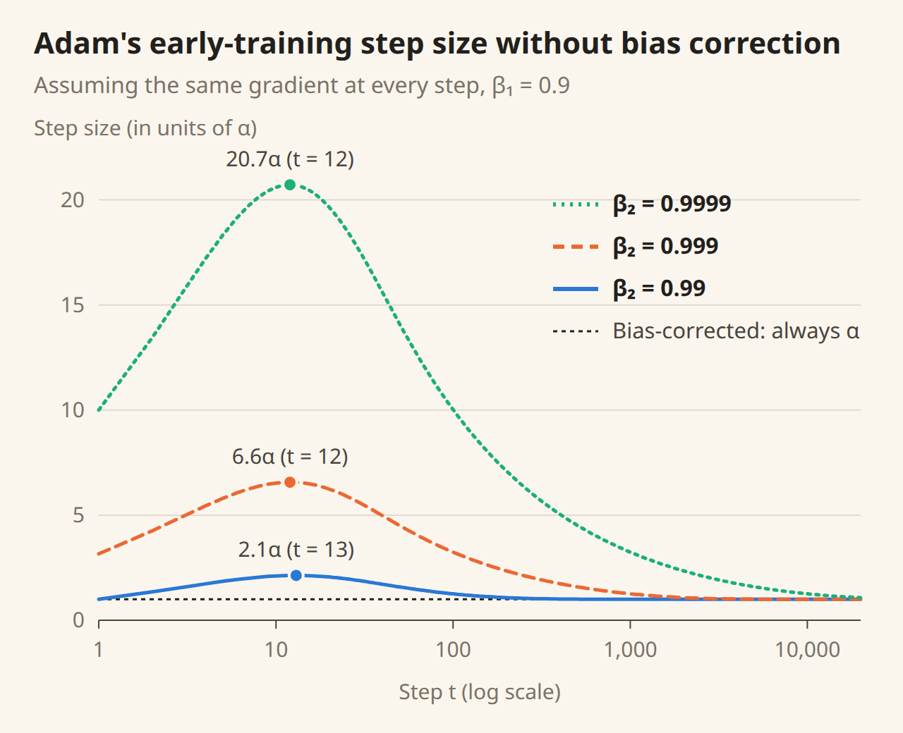
All three lines peak around steps 12 and 13. By then has built up to about 70% of its true value, while with , has built up only about 1%, which is still only a little over a tenth after the square root. The numerator has caught up; the denominator hasn't. With the peak is , and it takes over 1,700 steps to get back within ; with the peak is , and it takes over 17,000 steps.
Take momentum away as well (), and the uncorrected first step is , which at is . The learning rate is set to , yet the first step effectively uses .
This is exactly the situation the paper describes. Sparse gradients need a large to average over enough samples, and the closer gets to 1, the worse the uncorrected initial bias becomes.
How far one step goes
Section 2.1 goes on to analyze the update itself. Set for now; the effective step at each iteration is .
is "the mean of the gradient" divided by "the square root of the mean of the squared gradient." Since , the absolute value of this ratio usually doesn't exceed 1, so is roughly bounded by .
There is one exception. If a parameter's gradient has been 0 all along and suddenly has a value at this step, is about and about , and the ratio becomes . The bound the paper gives therefore has two cases:
Plugging in the defaults, is larger than , so the default setting falls into the first case, with a worst case of . This only happens for extremely sparse parameters; the paper says that when the sparsity is less extreme, the effective step will be smaller than this.
This property has three practical consequences.
- is the step size. It is roughly the distance moved in parameter space at each step, and the paper likens it to drawing a trust region around the current parameters. If we know roughly how far a good solution is from the initial values, we can estimate the order of magnitude of .
- It doesn't depend on the gradient's scale. Multiply the gradient by , and becomes times larger and becomes times larger, leaving the ratio unchanged. Multiply the loss function by 1000, and SGD's steps grow 1000-fold, while Adam isn't affected at all.
- Automatic annealing. The paper borrows the term "signal-to-noise ratio" for . Near an optimum, the gradient direction often flips back and forth, so the mean approaches 0 while the mean of the squares is still there; the ratio shrinks, and the step shrinks along with it.
Relation to AdaGrad and RMSProp
Section 5 puts Adam back into the family it came from and compares.
Compared with RMSProp, there are two differences. RMSProp with momentum first divides the gradient by the scale and then applies momentum to the result; Adam estimates the gradient's first and second moments separately and then divides one by the other. The other difference is bias correction.
The relationship with AdaGrad is more interesting. Set , let approach 0, and replace the learning rate with ; the bias-corrected becomes , and substituting this back into the update gives exactly AdaGrad. This correspondence holds only if bias correction is kept; without it, approaching 1 sends toward 0, and the update becomes infinite.
The paper also notes that can be viewed as an approximation of the diagonal of the Fisher information matrix, so Adam amounts to preconditioning with its inverse square root. Compared with natural gradient, which uses the inverse of the Fisher matrix directly, this approach is somewhat more conservative.
AdaMax
Section 7.1 is an extension. Adam scales by the norm of the gradient, and the authors generalize this to :
Large is numerically unstable, but if we let and set , only the largest term in the weighted sum survives, giving a very simple recursion:
is "a discounted record of the largest past gradient." If some step sees , becomes 10 and is then multiplied by 0.999 at every step, so a thousand steps later about 3.7 remains. It needs no bias correction, because is always at least the current and never has to creep up from 0. The bound on the step is simpler too, . The paper's suggested defaults are , with and the same as in Adam.
Section 7.2 also proposes an exponential moving average of the parameters, , again correcting the initial bias with .
Convergence proof
Section 4 analyzes Adam in the framework of online convex optimization. At each step the algorithm faces a convex function that isn't known in advance, and the yardstick is regret, the amount by which the cumulative loss exceeds that of the best fixed parameters in hindsight:
Theorem 4.1 comes with a long list of conditions: bounded gradients, bounded distances between iterates, , a learning rate decaying as , and also decaying over time as . Under these conditions, the paper obtains regret, so the average regret goes to 0.
In practice Adam is rarely run under these conditions. The learning rate is often constant or follows some other schedule, and is fixed at 0.9. The paper itself admits in Section 6.2 that this analysis doesn't apply to non-convex problems such as neural networks.
This theorem was later shown to be wrong. In 2018, Reddi, Kale, and Kumar pointed out that at one step, the proof in the appendix treats as if it could never be negative. This quantity is how "the inverse of the effective learning rate" changes over time; Adam's is a moving average that shrinks when the gradients shrink, so it can be negative. They also pointed out problems with Lemmas 10.3 and 10.4, and constructed a one-dimensional convex problem that satisfies the theorem's conditions, on which Adam converges to the worst possible point.
Discussion
The three experiments on logistic regression, multilayer perceptrons, and convolutional networks all use a batch size of 128, and the optimizers being compared start from the same initial parameters; hyperparameters such as the learning rate and momentum are searched over a dense grid, and the best setting is reported. The paper plots only loss curves, and for the first three experiments it states explicitly that these are training losses; there is no test accuracy. Keep this in mind when reading the figures, because what these experiments compare is who drives the training loss down faster.
Logistic regression
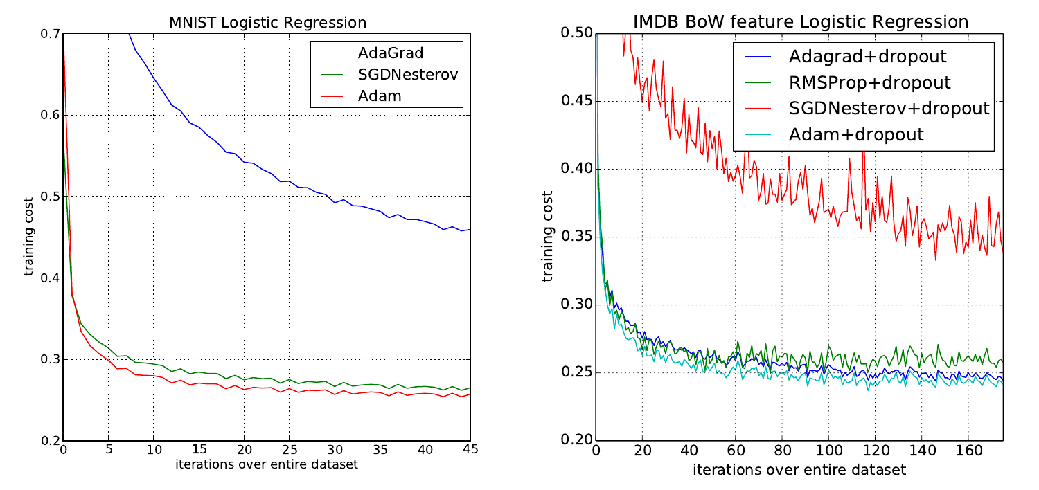
Logistic regression is a convex problem with no local minima to worry about, which makes it a clean setting for comparing optimizers. In this experiment the learning rate decays as , following the theory in Section 4.
The left panel is MNIST, classifying the raw 784-dimensional pixel vectors. Adam and SGD with momentum are about even, and both are much faster than AdaGrad.
The right panel is what Adam really sets out to prove. The authors turn IMDB movie reviews into bag-of-words vectors over the 10,000 most frequent words; each review uses only a few of those words, so the features are very sparse. To prevent overfitting, 50% dropout is applied to the features. Here AdaGrad is far ahead of SGD, and Adam is just as fast as AdaGrad. Adam has inherited AdaGrad's advantage on sparse features.
Multilayer perceptron
Next is a fully connected network with two layers of 1000 ReLU units each, again on MNIST. In the version with dropout, Adam's training loss is lower than that of AdaGrad, RMSProp, SGD with momentum, and AdaDelta.
For the version without dropout, which uses L2 weight decay instead, the authors also compare against SFO. SFO is a quasi-Newton method that operates on mini-batches and updates its curvature information at every step; it is 5 to 10 times slower than Adam, and its memory grows linearly with the number of mini-batches. Adam is faster whether measured in iterations or in wall-clock time, and since SFO assumes each sub-function is deterministic, it fails to converge once dropout is involved.
Convolutional network
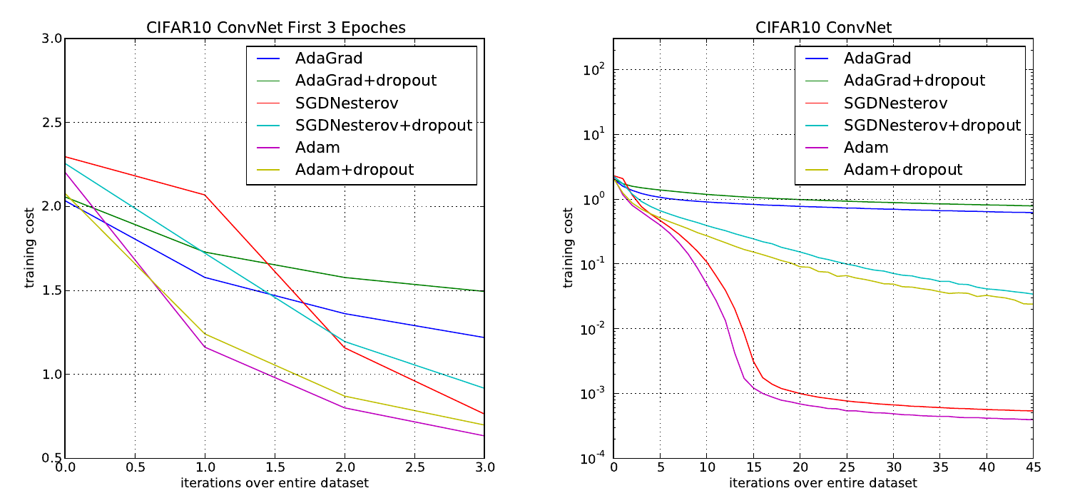
The network has three stages of convolutions with max pooling at stride 2, with 64, 64, and 128 channels, followed by a fully connected layer of 1000 ReLUs; the inputs are whitened, and dropout is applied to the input layer and the fully connected layer.
Over the first 3 epochs on the left, both Adam and AdaGrad drop quickly. Stretch it out to 45 epochs on the right, though, and AdaGrad stalls early, while Adam and SGD with momentum keep going down below .
The authors' explanation for this result is quite specific. They observed that after a few epochs of training, becomes so small that it is nearly 0, the denominator is dominated by , and the second moment no longer describes the geometry of the problem; what does the work in convolutional networks is mainly the first moment, which averages out mini-batch noise. Following this explanation through, when the denominator is dominated by , Adam behaves more like SGD with momentum, which also fits how close the two curves are. The authors are candid that Adam is only a marginal improvement over SGD with momentum, and that its benefit is in automatically adjusting the learning-rate scale for different layers, with no need to hand-pick a smaller learning rate for the convolutional layers.
is described as "a small constant to avoid division by zero," but once shrinks to the same order of magnitude, it is actually taking part in the update.
The bias-correction experiment
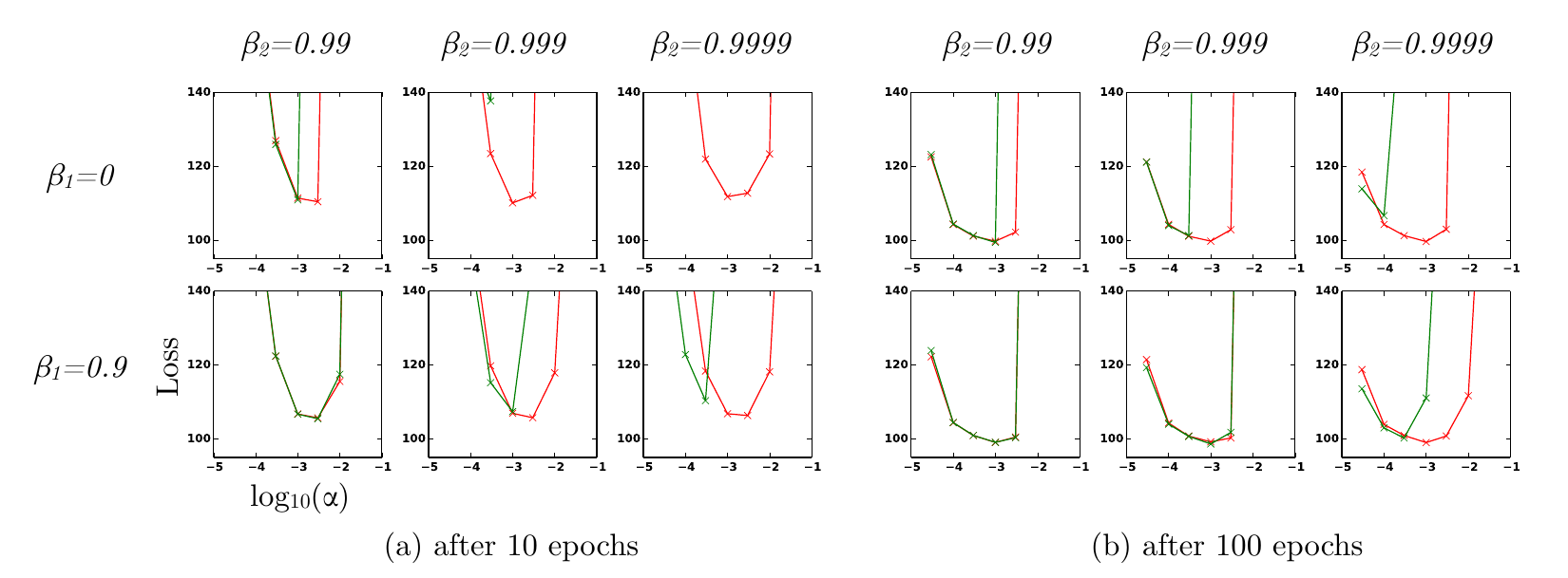
This is the figure in the paper that tests the design most directly. The authors train a variational autoencoder (VAE, with a single hidden layer of 500 softplus units and a 50-dimensional Gaussian latent variable), sweeping , , and from to . The paper treats Adam with bias correction removed as a form of RMSProp with momentum.
In each small plot, the horizontal axis is the learning rate and the vertical axis is the loss; red is with correction and green is without.
- In the column, the red and green lines roughly overlap; only in the row does the green line shoot off the plot first, at the largest learning rate. With this setting, the bias from skipping the correction disappears within one or two hundred steps and has little effect on training as a whole.
- Moving right to , the green line shoots off the plot already at the larger learning rates. The worst case is the first row of the left group, , where the green lines for and are almost entirely off the plot; without correction, the first step in these two cells is and , respectively.
- In the right group, trained to 100 epochs, the red line's lowest point is around 100 in all six plots. In the column, the red line bottoms out at ; at that same learning rate, the green line has already shot off the plot for and climbed to about 110 for . The red line has a much wider range of usable learning rates.
The authors conclude that when is close to 1, the lack of bias correction makes training unstable, especially in the first few epochs, and that the best results come from settings with a very small combined with bias correction. Across all the hyperparameters they swept, Adam was never worse than RMSProp.
The authors add one more observation. Late in training, hidden units specialize and the gradients become sparser, which is when the benefit of a large shows most clearly. In other words, a close to 1 is the setting we wanted all along, and bias correction lets us use it with confidence.
Where goes
Back to the difference between the two formulations from earlier. Algorithm 1 adds to the corrected , while the cheaper form adds to the uncorrected . Converting between them gives , and the two differ most early in training.
Different frameworks picked different forms. PyTorch follows Algorithm 1, with a default of eps=1e-8; Keras's documentation states that its epsilon is the paper's , with a default of 1e-7. When moving hyperparameters between these two frameworks, the thing called epsilon on each side is actually a different quantity.
This seemingly unimportant constant gets tuned in large-model training, too. OLMo 2 lowered AdamW's from to and reported that gradient norms early in training became lower and more stable as a result.
The years without bias correction
The derivation in Section 3 sounds like a minor detail, but it has a real-world sequel.
BERTAdam, the optimizer in BERT's official code, dropped those two bias-correction lines, and this version was then copied into widely used libraries such as Hugging Face Transformers (which only switched back to standard Adam in July 2019) and AllenNLP. In 2020, Zhang et al.'s "Revisiting Few-sample BERT Fine-tuning" traced why BERT fine-tuning is unstable on small datasets and found this to be one of the main causes.
They fine-tuned on four small datasets, RTE, MRPC, STS-B, and CoLA, with 50 random seeds each. Without bias correction, many fine-tuning runs never got off the ground; on RTE, for example, 48% of runs had an accuracy below 55%, close to random guessing. With bias correction restored, the variance of the results shrank substantially.
The reason is the same as in the step-size plot above. Fine-tuning on these small datasets usually takes fewer than a thousand steps, so the entire run sits in the stretch where the bias is largest. On MNLI, which trains for many more steps, the difference with and without correction falls within the margin of error (validation accuracy of 86.0 without correction and 85.9 with it).
Three questions that followed
Adam quickly became the default optimizer, and over the next few years, the challenges to it fell roughly along three lines:
- Convergence. This is the proof error mentioned earlier. Reddi et al. used an example with a large gradient once every three steps to show that "forgets" rare large gradients, and proposed AMSGrad, which keeps the historical maximum.
- Generalization. In 2017, Wilson et al. found on several vision and language tasks that Adam drives the training loss down quickly but often loses to well-tuned SGD on the test set.
- Regularization. Loshchilov and Hutter pointed out that in Adam, writing L2 regularization into the gradient is not equivalent to applying weight decay directly, and proposed AdamW.
Conclusion
Adam uses two exponential moving averages to estimate the mean and the mean square of the gradient, and dividing one by the other gives each parameter a step size of its own; it then uses to correct the bias from starting at 0, so that even the first step lands on the scale of . The paper's most convincing evidence is the VAE experiment, which shows that the closer is to 1, the more bias correction matters; the other experiments compare only training loss, and on convolutional networks its margin over SGD with momentum is small. The convergence theorem was shown to be wrong three years later.
If you're implementing Adam yourself, or reusing someone else's training code, first check whether those two bias-correction lines are still there, then check whether is added before or after bias correction, and what its value is. The fewer training steps you have, the more these two details affect the results; and when moving hyperparameters between frameworks, remember that the epsilon on each side may not be the same quantity.
In 2025, this paper won the ICLR Test of Time Award, seven years after its convergence proof was shown to be flawed. As for the author order, that still comes down to the coin.