Original paper
Accurate, Large Minibatch SGD: Training ImageNet in 1 Hour
- Publication
- Publication venue not yet verified
- First submitted to arXiv
- arXiv:1706.02677
Cite this paper · BibTeX
The citation identifies the linked source version. It cites the original paper and its authors.
@misc{optimizerslargeminibatchsgd2017,
  title = {{Accurate, Large Minibatch SGD: Training ImageNet in 1 Hour}},
  author = {Priya Goyal and Piotr Dollár and Ross Girshick and Pieter Noordhuis and Lukasz Wesolowski and Aapo Kyrola and Andrew Tulloch and Yangqing Jia and Kaiming He},
  year = {2017},
  eprint = {1706.02677},
  archivePrefix = {arXiv},
  url = {https://arxiv.org/abs/1706.02677}
}
Training ResNet-50 on 8 Tesla P100s with a batch size of 256 takes 29 hours to get through 90 epochs of ImageNet.
In June 2017, a team at Facebook moved the same model onto 256 GPUs, raised the batch size to 8,192, and finished training in one hour, with a top-1 validation error only 0.14 percentage points off the original. The author list includes Ross Girshick, Piotr Dollár, and Kaiming He, as well as Yangqing Jia, the creator of Caffe.
With 32 times the GPUs cutting the time 29-fold, it looks like a result achieved by piling on hardware. Yet this technical report spends most of its pages on everything other than the hardware, including how to adjust the learning rate when the batch becomes 32 times larger, why things go wrong at the start of training, how BatchNorm should be computed, and a handful of implementation details that still run when you get them wrong, only with worse results.
Defining the problem
In synchronous distributed SGD, workers (here, GPUs) each compute gradients on samples, sum the gradients, and all update their parameters with the same result. Each step sees samples.
To keep every card busy, can't be too small, so the more GPUs there are, the larger the total batch. For the same 90 epochs, a batch 32 times larger means 32 times fewer updates.
Large batches had a poor reputation at the time. In 2014, Krizhevsky used a learning rate that scaled linearly with the batch size, but when the batch grew from 128 to 1,024, the error went up by 1 percentage point. Keskar et al. (2017) argued that large batches converge to sharp minima and generalize worse. Others had trained with a batch of 5,120 without losing accuracy, but without giving an adjustment rule that avoided hyperparameter search.
This paper asks whether, as the batch grows from 256 upward, a single simple rule, with no other hyperparameters retuned, is enough to keep the accuracy of small batches. And if not, where does it break?
Solving the problem
The linear scaling rule
The authors' rule is a single sentence, multiply the batch by , and multiply the learning rate by too. Every other hyperparameter, weight decay included, stays the same.
Why multiply by ? Let's walk through . One step of mini-batch SGD is:
Take two consecutive steps with two mini-batches and , where the second step's gradient is computed at :
Now merge the two mini-batches into one large batch of size and take a single step with learning rate :
The two equations differ in only two places, whether the second mini-batch's gradient is computed at or at , and the coefficient in front. If the gradient doesn't change much after the parameters take a step, that is, , then for the two to be equal we need , which means . Generalized to mini-batches, this gives the paper's Eqs. (3) and (4), and .
The authors themselves call this a strong assumption, and point out at least two situations where it clearly fails. The first is the beginning of training, when the network changes rapidly and the gradients of neighboring steps differ a lot. The second is that the batch can't be made arbitrarily large; results stay stable over a wide range, but beyond a certain point, accuracy degrades rapidly, and on ImageNet that point is around 8k.
Warmup takes care of the first situation.
Warmup
The ResNet paper had used a constant warmup, running the first few epochs at a small fixed learning rate. The authors tried this on an 8k batch, using for the first 5 epochs and then jumping straight to , and found it wasn't enough; the moment training switched out of the low learning rate, the training error spiked.
So they switched to a gradual warmup, starting from and adding a fixed amount at every step so that the learning rate reaches exactly after 5 epochs, and then rejoining the original schedule.
Let's work out the numbers for an 8k batch. The ImageNet training set has about 1.28 million images, so an epoch is about 156 steps and 5 epochs about 780 steps. The learning rate has to climb from 0.1 to 3.2, adding roughly 0.004 per step. The authors also mention that the results are not sensitive to the length of the warmup.
BatchNorm's batch
BatchNorm computes the mean and variance within a batch, so each sample's loss no longer depends only on itself but also on the other samples in the same batch. The authors spell this out in Eq. (5). With BN, the training set can be thought of as "all subsets of size ," and each such subset counts as one independent sample.
This means that BN's batch size is part of the definition of the loss function. Change , and the randomness of the BN statistics changes with it, so the optimization target becomes a different one. That's why the authors fix per worker and only increase when adding GPUs; the BN statistics are also computed separately within each worker, not synchronized across workers. This saves communication, and more importantly, it makes the experiments with different batch sizes optimize the same objective. The paper also specifically says that if you want to change , you should tune it as a hyperparameter of BN, not as a parameter of distributed training.
Four implementation pitfalls
Section 3 lists four details that "still train when written wrong, only with higher error than expected," each summarized as a Remark.
Weight decay. Weight decay is really the gradient of an L2 term in the loss. Write the per-sample loss as , and the SGD update becomes Eq. (8):
In practice, backpropagation only computes the cross-entropy term, and is added separately. So multiplying the cross-entropy loss by only scales up the latter term and leaves the weight decay term untouched, which is not the same as multiplying the learning rate by . That is Remark 1. Scaling the cross-entropy loss and scaling the learning rate are two different things.
Momentum correction. There are two common ways to write momentum SGD. The reference form is Eq. (9), where the momentum buffer accumulates only gradients, and the learning rate is applied when updating the parameters:
The other form is Eq. (10), which absorbs the learning rate into the buffer by setting :
With a fixed learning rate, the two are exactly equivalent. Once the learning rate changes, they're not. What stores is history already multiplied by the old learning rate, so to stay consistent with Eq. (9), it has to be multiplied by before the update; the authors call this ratio the momentum correction. They found that when the learning rate is raised sharply () without the correction, the history term is too small and training becomes unstable; when the learning rate goes down, the correction matters less. That is Remark 2. With the Eq. (10) form, apply momentum correction whenever you change the learning rate.
Gradient aggregation. The correct large-batch gradient is the sum of the gradients over samples, divided by . Each worker's loss layer usually already averages over its own samples, while allreduce performs a sum, not an average, so a factor of is still missing. The authors suggest putting this directly into the loss, which only scales the gradient of the loss with respect to its input and saves you from scaling the entire gradient vector. That is Remark 3. Each worker's loss should be divided by the total batch , not by its own . The paper also warns against making the two cancel out by not multiplying the learning rate by and dividing the loss by only ; weight decay then comes out wrong, for the reason given in Remark 1.
Data shuffling. SGD theory assumes random sampling every time, while in practice the training set is shuffled once per epoch. For a fair comparison with a shuffling baseline, only one random permutation is generated per epoch, then split into parts for the workers. That is Remark 4. If each worker shuffles on its own without coordination, the behavior can differ noticeably and contaminate the experimental conclusions.
Communication
To go beyond the 8 cards in one server, gradients have to be aggregated over the network. Gradients of different layers don't depend on each other, so as soon as one layer's gradient is ready, its allreduce can start while the next layer is still being computed, hiding the communication behind backpropagation.
Allreduce runs in three stages. First the buffers of the 8 cards within a server are summed, then the sums are added up across servers, and finally the result is broadcast back to every card. For the cross-server part, the authors implemented two algorithms, recursive halving/doubling and ring; on 32 servers (256 cards), the former is 3 times faster than the latter. All of this lives in Facebook's open-source Gloo, running with Caffe2.
The hardware is Facebook's Big Basin servers, each with 8 P100s interconnected by NVLink, and ordinary 50 Gbit Ethernet between servers. The authors estimated the bandwidth. ResNet-50 has about 25 million parameters, or 100 MB; backpropagation on a single P100 takes about 120 milliseconds; allreduce network traffic is about 2 times the data size, so the peak requirement is 200 MB / 0.125 s = 1,600 MB/s, about 12.8 Gbit/s, or about 15 Gbit/s with overhead, which 50 Gbit can handle.
Discussion
Experimental setup
The main benchmark is top-1 validation error on ImageNet-1k. The model is the fb.resnet.torch version of ResNet-50 (with stride 2 on the 3×3 convolution), with Nesterov momentum 0.9 and weight decay 0.0001, not applied to BN's and . Every batch size is trained for 90 epochs, with a reference learning rate of , divided by 10 at epochs 30, 60, and 80; with and , this is the original 0.1.
There's one more detail in the initialization. The of the last BN in each residual block is initialized to 0, so the signal initially passes only through the shortcut. The authors found this helps for all models, and especially for large batches.
Randomness is handled with care, too. For each model, they take the median error over the last 5 epochs, then report the mean and standard deviation over 5 independent training runs. The baseline (batch 256) error is 23.60% ± 0.12. Batches of 12k and above were limited by hardware and were simulated on a single server with gradient accumulation; the authors state that they verified the results are equivalent to true distributed training.
Three kinds of warmup
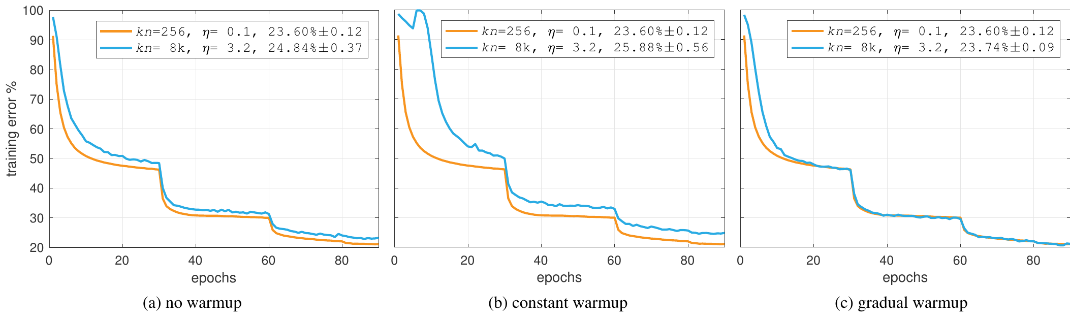
In all three panels, the orange line is the batch-256 baseline and the blue line is the 8k batch with learning rate 3.2. The percentages in the legends are validation errors.
- No warmup (a): the blue line stays above the orange line from start to finish. The final training error is about 2.1 percentage points higher, and the validation error is about 1.2 percentage points higher (24.84%). From this the authors conclude that the higher validation error comes mainly from the training error, not from overfitting.
- Constant warmup (b): the low learning rate in the first 5 epochs does bring the error down, but as soon as it switches to 3.2, the error shoots up and never fully catches up afterward, making the validation error the worst of the three (25.88%).
- Gradual warmup (c): the blue line starts out higher because the learning rate is small, then merges with the orange line after about 20 epochs, with a validation error of 23.74%, only 0.14 percentage points from the baseline, when the standard deviation itself is about 0.1.
That even the training curves line up is a point the paper stresses repeatedly. From this the authors argue that the difficulty of large batches is mainly one of optimization; as long as the training error keeps up, there's no sign of worse generalization within this range.
8k is the ceiling
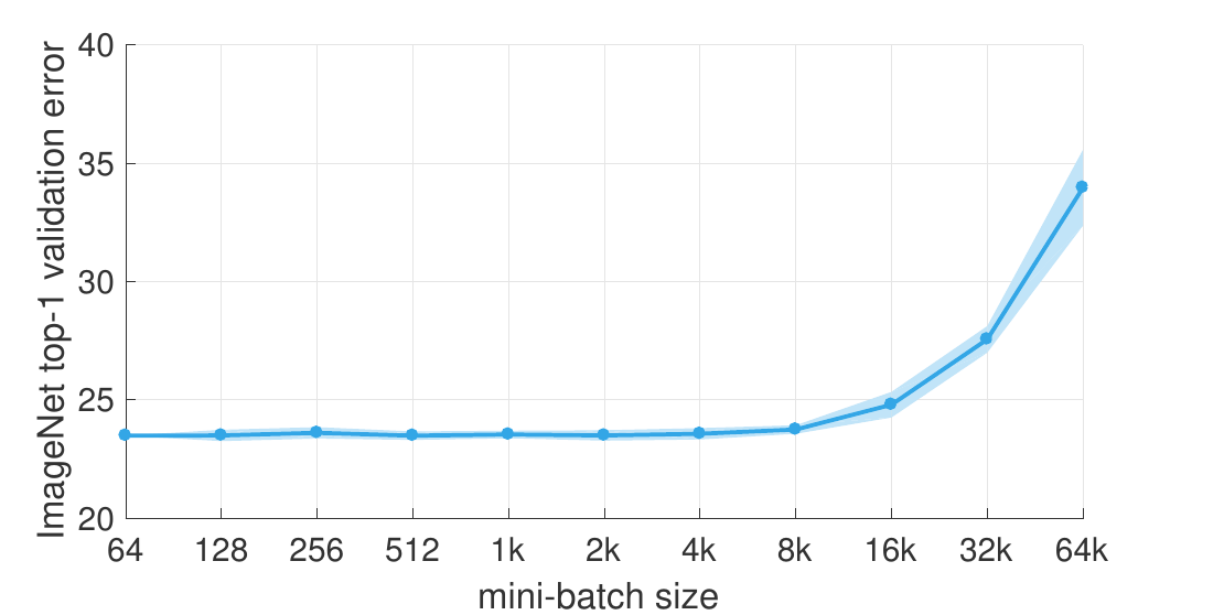
Every batch uses the linear scaling rule, and batches larger than 256 also get 5 epochs of gradual warmup. From 64 to 8k, the error is nearly a flat line; past 8k it starts to rise, to 24.79% at 16k, 27.55% at 32k, and 33.96% at 64k. Beyond that, training with the linear rule simply diverges.
The training curves show the difference too.
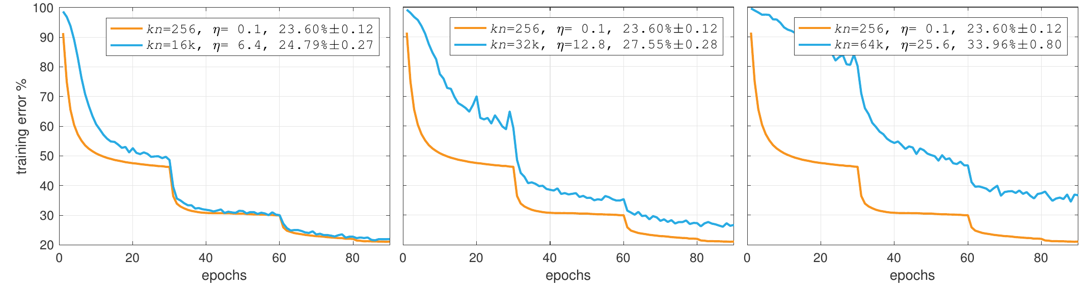
For batches up to 8k, the training curves overlap with the baseline apart from the warmup stretch. At 16k and above, the two lines are clearly apart throughout training. The authors therefore suggest using the training curve as an early indicator when evaluating a new setting; if the curves don't match, the final validation error usually won't either.
ResNet-101 behaves similarly. Its error with an 8k batch is 22.36%, 0.28 percentage points higher than the 22.08% with a 256 batch, and the authors consider 8k to already be at the edge for ResNet-101; training it on 256 P100s takes 92.5 minutes.
Does the ceiling go up as the data grows? The authors switched to ImageNet-5k, adding 4,000 classes from ImageNet-22k for a total of 6.8 million images, about 5 times the original, while still evaluating 1,000-class classification on the ImageNet-1k validation set. The shape of the error curve is almost identical to ImageNet-1k's, with an 8k batch only 0.26 percentage points higher than 256 (25.83% to 26.09%), and the turning point doesn't move later. With 5 times the data, the usable batch size didn't grow along with it.
Other scaling rules
Is the linear rule really the best? The authors tried several learning rates at both 256 and 8k:
| Batch | Learning rate η | top-1 error |
|---|---|---|
| 256 | 0.05 | 23.92 |
| 256 | 0.10 | 23.60 |
| 256 | 0.20 | 23.68 |
| 8k | 0.05 · 32 | 24.27 |
| 8k | 0.10 · 32 | 23.74 |
| 8k | 0.20 · 32 | 24.05 |
| 8k | 0.10 | 41.67 |
| 8k | 0.10 · √32 | 26.22 |
Compiled from Table 2a of the paper; ResNet-50, mean of 5 runs (%).
The best value for the 256 batch is 0.1, and the best for the 8k batch is 0.1 × 32 = 3.2, exactly what the linear rule says. When the learning rate isn't scaled up at all (0.10), the error is as high as 41.67%. Krizhevsky derived a square-root rule from the standard deviation of the gradient estimate; using with the same gradual warmup, the error is still 26.22%.
The 8k batch is also more sensitive to the learning rate than the 256 batch. Changing the multiplier from 0.1 to 0.05 or 0.2 makes a difference of only 0.1 to 0.3 percentage points for the 256 batch, but 0.3 to 0.5 percentage points for the 8k batch. The authors' advice is that in practice, you shouldn't choose a batch size close to the breaking point.
γ = 0 in residual blocks
Initializing the of the last BN in each residual block to 0 lowers the error from 23.84% to 23.60% for the 256 batch and from 24.11% to 23.74% for the 8k batch; the larger batch benefits more, which the authors take as further evidence that large batches are more susceptible to optimization difficulties. This trick later made it into torchvision, whose ResNet constructor has a zero_init_residual parameter; the code comment cites this paper and says it improves results by 0.2 to 0.3 percentage points.
Transfer to detection and segmentation
ImageNet accuracy usually isn't the end goal; what people care about is whether the pre-trained features work for other tasks. The authors used ResNet-50 models pre-trained with batches from 256 to 16k to initialize Mask R-CNN for object detection and instance segmentation on COCO. They pre-trained 5 models for each batch size, training 35 Mask R-CNNs in all, with every other hyperparameter taken from the original Mask R-CNN paper.
| Pre-training batch | top-1 error | box AP | mask AP |
|---|---|---|---|
| 256 | 23.60 | 35.9 | 33.9 |
| 1k | 23.53 | 35.9 | 33.9 |
| 4k | 23.56 | 35.8 | 33.8 |
| 8k | 23.74 | 35.8 | 33.9 |
| 16k | 24.79 | 35.1 | 33.2 |
Compiled from Table 3a of the paper, selected rows; COCO minival, mean of 5 runs (%).
As long as the ImageNet error holds (up to 8k), the detection and segmentation AP are virtually identical; at 16k the ImageNet error goes up, and COCO AP drops by 0.7 to 0.8 percentage points along with it.
The linear rule itself also works for Mask R-CNN. Batches mean something different for Mask R-CNN than for classification; the backbone takes 2 images per card, and each image contributes 512 RoIs for the three losses of classification, box regression, and mask. The authors trained on 1, 2, 4, and 8 cards, scaling the learning rate linearly with the number of cards (0.0025 to 0.02), and got box AP between 35.6 and 35.7 and mask AP between 33.5 and 33.7, with practically no difference. The paper also notes that Mask R-CNN's default 8-card setup had already been quietly applying this rule all along.
How fast
Going from a batch of 256 to 11k (44 times larger), the time per step increases by only 12%; per epoch, that takes training from over 16 minutes down to about 30 seconds, using 352 cards (44 servers) at that point. Compared with ideal extrapolation from the 8-card baseline, scaling from 8 cards to 256 cards is about 90% efficient, and this is on ordinary Ethernet.
What came after
The 8k ceiling was soon challenged. Two months later, You et al. stated flatly in the abstract of the LARS paper that the linear scaling plus warmup recipe isn't general enough and that training can diverge; they switched to adjusting the learning rate layer by layer and pushed ResNet-50's batch to 32k.
Shallue et al. (JMLR 2019) systematically measured the relationship between batch size and the number of training steps across 35 workloads. They found that the perfect-scaling regime, where "doubling the batch halves the steps," varies enormously between tasks, and that the optimal learning rate doesn't necessarily follow the linear or square-root rule; they also found no evidence that large batches hurt generalization. Taken together, the linear scaling rule is best treated as a rule of thumb within the perfect-scaling regime; outside that range, the hyperparameters have to be retuned.
Warmup, meanwhile, stuck around, and spread beyond large batches. Transformers trained with Adam almost always need warmup, and later Pre-LN and RAdam each offered an explanation for this.
Conclusion
This paper relies on three things to push ResNet-50's batch from 256 to 8k, namely scaling the learning rate linearly with the batch, a gradual warmup over the first 5 epochs, and computing BN on a fixed 32 samples per card. The 8k batch's error of 23.74% differs from the 256 batch's 23.60% by about one standard deviation, the training curves line up, and transfer to detection and segmentation doesn't get worse; past 8k, the same recipe starts to fail.
When you actually go from 1 card to 8 cards, the most useful part of this paper turns out to be Section 3. After scaling the learning rate with the number of cards and adding warmup, you still need to check whether the loss is divided by the total batch or the per-card batch, whether you scaled the learning rate or only the loss (the latter throws off weight decay), and whether your framework's momentum buffer has the learning rate multiplied into it. Get any of these wrong, and the model will still converge, just with somewhat higher error, which is hard to notice.
Five months later, a paper from Preferred Networks was titled "Extremely Large Minibatch SGD: Training ResNet-50 on ImageNet in 15 Minutes," using 1,024 P100s and a 32k batch. (The title is almost copied word for word, with Accurate swapped for Extremely and 1 Hour for 15 Minutes.)