Original paper
On the Convergence of Adam and Beyond
- Publication
- ICLR 2018Conference
- First submitted to arXiv
- arXiv:1904.09237
Cite this paper · BibTeX
The citation identifies the linked source version. It cites the original paper and its authors.
@misc{optimizersamsgrad2019,
  title = {{On the Convergence of Adam and Beyond}},
  author = {Sashank J. Reddi and Satyen Kale and Sanjiv Kumar},
  year = {2019},
  eprint = {1904.09237},
  archivePrefix = {arXiv},
  url = {https://arxiv.org/abs/1904.09237}
}
Let's start with a little game.
The parameter has to stay between and . Every three steps make up one round; the loss at the first step is , and at the second and third steps it is . A round adds up to , so the smaller the better, and the answer is .
The gradients are easy to work out, at the first step and at the next two. SGD takes one net step in the negative direction each round and ends up at .
Adam ends up at , the worst point in the whole interval.
This example comes from Sashank Reddi, Satyen Kale, and Sanjiv Kumar at Google. They used it to prove that the convergence theorem in the original Adam paper is wrong, and then, working from where the proof goes wrong, derived a fix that changes a single line, AMSGrad.
Defining the problem
Adam's claimed convergence
The Adam paper analyzes convergence in the framework of online convex optimization. At each step, the algorithm first picks a parameter , and only then sees this step's convex loss function . The yardstick is regret, the amount by which the cumulative loss exceeds that of "the best fixed parameter in hindsight":
If the average regret goes to 0, then on average the algorithm has caught up with the best fixed solution. Theorem 4.1 of the Adam paper claims that under conditions including bounded gradients, , and a learning rate of , Adam's regret is and its average regret goes to 0.
The game at the top of this note is exactly an online convex optimization problem. Each is a linear function, and the feasible set is . Adam stays at and incurs a fixed amount of extra loss every round compared with , so its average regret never goes to 0.
Can the effective learning rate grow?
Reddi et al. point to one particular quantity. Write the various adaptive methods in a common framework, where each update is , so that is the actual learning rate of each parameter. Now look at how its inverse changes over time:
For SGD, is fixed and decreases. For AdaGrad, is the average of past squared gradients, and paired with , what actually sits in the denominator is the sum of squared gradients, which only ever grows. For both methods is never negative, and the learning rate can only shrink.
Adam and RMSProp use exponential moving averages. As soon as recent gradients get smaller, shrinks with them and the learning rate grows instead, so can be negative.
The paper opens by describing what people see in practice. In problems with very large output spaces, some mini-batches bring large, informative gradients, but they show up only rarely; the exponential moving average makes their influence fade quickly, and training converges poorly. This paper sets out to turn that intuition into a provable counterexample.
Solving the problem
Counterexample: a large gradient every three steps
Theorem 1 of the paper is the general version of the opening game. The loss functions are, in order,
The gradients over one round sum to , and the optimum is . Adam is set to , , , with ; these parameters satisfy the Adam paper's requirement that . The paper's appendix proves by induction that, starting from , returns to at the end of every round.
Why? Take , which makes , and compute one round directly. After a few rounds settles into a fixed cycle, and the table below shows one round of that cycle. The last two columns are , where a positive value pushes toward and a negative value pushes it toward . The actual update also gets multiplied by , but is about the same for the three steps within a round, so we'll ignore it for now:
| Step | Adam | AMSGrad | ||
|---|---|---|---|---|
| 1 | 8.21 | |||
| 2 | 1.72 | |||
| 3 | 1.07 | |||
| Round |
Computed for this note with , , , the setting of Theorem 1. AMSGrad's denominator uses the largest so far, which is 8.21.
Look at the Adam column first. The gradient at the first step is , but it also pumps up to 8.21, and , so the large gradient gets shrunk by nearly a factor of 3. When the paper says the large gradient is scaled down "by a factor of almost ," this is what it means. For the next two steps the gradient is only , and falls back to 1.72 and then 1.07, keeping only a tenth of its value at each step; the learning rate grows nearly threefold within two steps, and the two small gradients together push by . Over the round, the net effect is a move of in the wrong direction.
This is what looks like in concrete terms. Two steps later, the lesson taught by the large gradient is mostly forgotten.
Running this setup with for three hundred thousand steps, Adam stays at with an average regret of , exactly the lower bound given in the paper; under the same conditions, AMSGrad reaches .
The paper adds a few more points. The example holds just as well with a constant step size . Adding to the denominator doesn't rescue Adam either; Theorem 6 in the appendix constructs a similar counterexample for any . On the same problem, SGD and AdaGrad both have average regret going to 0.
With the values people actually use
is far too contrived; in practice, is always close to 1. The paper goes on to prove two stronger results.
Theorem 2 says that as long as (which nearly every practical setting satisfies), there exists an online convex problem on which Adam's average regret doesn't go to 0. The construction is the same, except that the period stretches from 3 to ; once every steps there is a gradient of , and all the rest are . has to be large enough that 's memory can't make it through a full period.
How large is large enough? The appendix lists three conditions, one of which is . Plugging in numbers ourselves, must be at least 3,218 for (Appendix B also requires to be even; the inequality alone gives 3,217) and at least 42,622 for . In other words, a gradient more than forty thousand times larger than usual, showing up once every forty-some thousand steps.
Theorem 3 moves to stochastic optimization. Each step is sampled independently, seeing with probability and otherwise. The expected loss is and the optimum is still , but when is large enough, the expected displacement of Adam at each step is positive, and the parameter drifts away from the optimum.
The authors conclude that to avoid this behavior, , , and would all have to depend on the problem; high-dimensional problems might even need a separate set for each dimension, which defeats the whole point of adaptive methods needing no tuning. They admit the examples are contrived, but argue that similar phenomena in real settings would at least slow convergence down.
Where the proof goes wrong
With a counterexample in hand, we know some step in Adam's original proof has to fail. In Section 4 and Appendix D, the paper points out that Adam's proof assumes is positive semi-definite, that is, that the learning rate never grows; this assumption doesn't hold for Adam. In addition, Lemmas 10.3 and 10.4 in Adam's proof also have problems.
The learning rates of SGD and AdaGrad are non-increasing to begin with, so they never run into this. This observation points straight to the fix.
AMSGrad
Since the problem is that can shrink, let the denominator remember the historical maximum:
The only difference from Adam is the third line. is still updated as an exponential moving average, so its estimate of the gradient scale still looks only at the recent past; but the actually used as the denominator never decreases, so the learning rate is non-increasing and is guaranteed to be positive semi-definite. The extra cost is just one vector the same size as the parameters.
Go back to the AMSGrad column of the table above. The denominator stays at 8.21, the two gradients each push by only , and the net effect over a round becomes a move of in the right direction.
The authors compare it with Adam and AdaGrad in one scenario. Suppose that at some step , meaning this step's gradient is smaller than the recent average:
- Adam aggressively increases the learning rate, which is exactly what sank it in the counterexample above;
- AdaGrad slightly decreases the learning rate, and over the long run the learning rate can get so small that the parameters barely move;
- AMSGrad neither increases nor decreases it.
The convergence guarantee for AMSGrad (Theorem 4) reuses the Adam paper's analysis framework with the problem above fixed. The conditions are , , , and a bounded feasible-set diameter and bounded gradients, and the regret bound picks up an extra ; the paper writes that choosing , or the milder , guarantees regret.
Two details are worth noting. The proof needs to decrease over time, but the authors also state that in practice is usually kept constant. And the Adam in this paper has bias correction removed; a footnote says this is for simplicity and that the counterexample argument applies equally to the corrected version. AMSGrad's Algorithm 2 has no bias correction either.
The paper also offers another route, AdamNC, which keeps the structure the same but lets increase over time. With , is exactly the average of all past squared gradients, which amounts to AdaGrad with momentum.
Discussion
Synthetic experiments
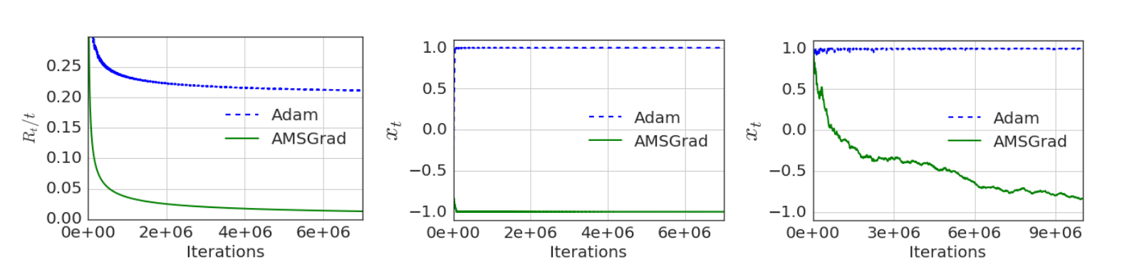
The experiment uses a scaled-up version of the counterexample. Once every 101 steps the loss is , and for the other 100 steps it is ; the gradients over one period sum to , and the optimum is still . This time the usual and are used, with the same parameters for both methods.
The left panel is the average regret. Adam's blue dashed line flattens out around 0.21 and stops falling, while AMSGrad's green line falls to near 0. The middle panel shows the parameter itself, with Adam at and AMSGrad at .
The right panel is the stochastic version, where each step sees with probability 1% and otherwise. Adam again stays at . AMSGrad moves down slowly; at ten million steps it is at roughly , still short of .
Real data
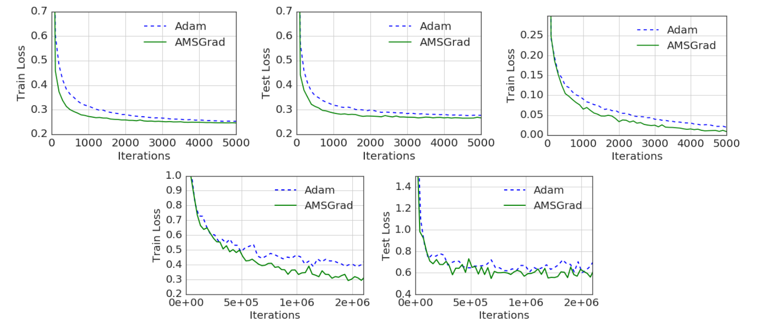
There are three real-data experiments, all with a batch size of 128 and , with chosen from :
- Logistic regression on MNIST (top row, left and middle). A convex problem, so the learning rate decays as as the theory prescribes, with and chosen by grid search. AMSGrad's training and test losses are both slightly lower, and the authors also mention that it is less sensitive to changes in its parameters.
- A one-hidden-layer network on MNIST (top row, right). 100 ReLUs and a constant learning rate. AMSGrad's training loss stays slightly below Adam's the whole way.
- CIFARNET on CIFAR-10 (bottom row). Two layers of 64-channel convolutions, followed by fully connected layers of 384 and 192 units, with max pooling, local response normalization, and dropout in between. The gap in training loss is the most visible, roughly 0.3 versus 0.4; the test loss of both is around 0.6, with AMSGrad slightly lower.
Keep the scope of these results in mind. The figures show only loss, not accuracy (the text says AMSGrad's accuracy is also better, but gives no numbers); each curve appears to be a single run, without error bars; and the models are all small. In their own list of contributions, the authors call this a preliminary empirical study.
The practical response
AMSGrad was quickly added to the major frameworks. Adam in both PyTorch and Keras has an amsgrad parameter, off by default.
Once people actually tried it, the feedback was lukewarm. In a July 2018 post, fast.ai's Sylvain Gugger and Jeremy Howard compared it on a Wide ResNet on CIFAR-10, ResNet-50 fine-tuned on Stanford Cars, and AWD-LSTM and QRNN language models on WikiText-2, writing that amsgrad consistently failed to bring any gain in accuracy or any other relevant metric, and calling it "very disappointing."
AMSGrad's own proof was later found to have a problem too. In 2019, Phuong and Phong pointed out that its proof treats and as if they were equal, the same slip found in Adam's original proof; they gave a new proof and also proposed another variant, AdamX.
Does Adam converge after all?
The counterexample stands, and yet Adam really does work well in practice. How do the two fit together? The answers from several follow-up works differ in what they fix first:
| Work | What is fixed first | Conclusion |
|---|---|---|
| Reddi et al. 2018 | Pick first, then construct the problem | Adam can fail to converge |
| Zhang et al. 2022 | Give the problem first, then pick | Converges if is large enough |
| ADOPT 2024 | Change the algorithm | Converges for any |
Zhang et al. 2022 put a finger on the question of order. Reddi et al. fix first and then construct a bad problem for that choice; as computed above, needs a period of more than forty thousand steps. In practice, though, the problem is there first, and then we tune the hyperparameters. They prove that for a fixed problem, as long as is large enough (with a threshold that depends on the problem) and , Adam with its update rule unchanged converges to a neighborhood of critical points whose size is proportional to the variance of the stochastic gradients; under stronger conditions it converges to the critical points themselves. This analysis targets non-convex finite-sum problems with the samples randomly reshuffled every epoch, doesn't need the bounded-gradient assumption, and covers the default . Conversely, when is too small, there is a large region of that diverges.
Around the same time, Défossez et al. gave a short convergence proof for smooth non-convex problems with bounded gradients, and also pointed out that Adam with default parameters, strictly speaking, does not converge, behaving more like SGD with a constant step size.
ADOPT 2024 takes a fresh look at AMSGrad. It points out that the convergence proofs for AMSGrad on non-convex problems all assume uniformly bounded stochastic gradients, and that models which inject Gaussian noise into their gradients, such as variational autoencoders and diffusion models, don't satisfy this condition. The trouble lies in taking the maximum, whose expectation is hard to control. ADOPT instead normalizes the current gradient with the previous step's , so the denominator doesn't contain the current gradient, and it normalizes first and accumulates momentum afterward. Assuming only that the gradient's second moment is finite, it achieves an convergence rate for any .
One last footnote. A July 2026 preprint, "On the Convergence of Adam, Revisited," claims that in the same online setting as Reddi et al., even the condition isn't needed, and that for any one can find an example where Adam's average regret doesn't vanish, still using a three-step cycle with slopes ; the result also extends to variants such as AdamW and Muon. This doesn't contradict Zhang et al.'s positive result, since the two answer the question in opposite orders.
Conclusion
Using a linear function with three-step rounds, this paper proved that Adam's original convergence theorem is wrong, and traced the problem to the exponential moving average allowing the learning rate to grow. AMSGrad uses the historical maximum as the denominator, which makes the learning rate non-increasing and restores the convergence guarantee for convex problems. The gains on real data are small, the experiments only go as far as a preliminary study, and later independent tests mostly saw no benefit. What this paper left to later research is the angle of analysis, along with the question of which side gets fixed first.
In practice, amsgrad=True is just a switch. If you suspect your data has rare but important large gradients, you can put it on the list to compare, alongside raising ; the former adds only one parameter-sized state, and the latter adds no cost at all. Zhang et al. proved that a large region diverges when is too small. Going by that result, if you lowered to make the optimizer react faster and training becomes unstable, the first thing to do is move it back close to 1.
The little three-step game, for its part, never retired. Eight years later it's still the same , only this time without even assuming , and it drags AdamW and Muon along for the ride.