Original paper
Decoupled Weight Decay Regularization
- Publication
- ICLR 2019Conference
- First submitted to arXiv
- arXiv:1711.05101
Cite this paper · BibTeX
The citation identifies the linked source version. It cites the original paper and its authors.
@misc{optimizersadamw2017,
  title = {{Decoupled Weight Decay Regularization}},
  author = {Ilya Loshchilov and Frank Hutter},
  year = {2017},
  eprint = {1711.05101},
  archivePrefix = {arXiv},
  url = {https://arxiv.org/abs/1711.05101}
}
The two lines of PyTorch below have the same parameter name and the same numbers:
torch.optim.Adam(model.parameters(), lr=1e-3, weight_decay=1e-2)
torch.optim.AdamW(model.parameters(), lr=1e-3, weight_decay=1e-2)
The first line treats 1e-2 as the coefficient of L2 regularization, adds it into the gradient, and hands the result to Adam; the second multiplies the parameters directly by at every step, independently of the gradient. The two train different models.
When Ilya Loshchilov and Frank Hutter of the University of Freiburg pointed out this difference in November 2017, the common framework implementations all used the first version, and they all called it weight decay.
Their claim is that this explains a large part of why Adam generalizes worse than SGD on image classification.
Defining the problem
Two kinds of "decay"
Weight decay, as Hanson and Pratt defined it in 1988, multiplies the weights by a number slightly less than 1 at every step before applying the gradient update (the paper's Eq. 1):
L2 regularization instead adds a term to the loss function, whose gradient is . With an SGD update:
Compare this with the previous equation, and as long as , the two are exactly the same. This is the paper's Proposition 1, and it is why people have long used the two terms interchangeably.
But this equality hides something that is often overlooked. If a problem has a best amount of decay , then the best L2 coefficient is tied to the learning rate; change the learning rate, and the L2 coefficient has to change with it. Even in SGD, these two hyperparameters are coupled.
What about Adam?
Adam divides the gradient by . If L2 is written into the gradient, the term gets divided along with it.
In May 2017, Wilson et al. found that Adam generalized worse than SGD on several tasks, and the best image classification results at the time were all still trained with SGD plus momentum. Several explanations for this gap had been proposed, such as sharp minima or problems inherent to adaptive methods. This paper offers another, more concrete hypothesis, that the problem may lie in the "weight decay" implemented in frameworks, which inside Adam isn't weight decay at all.
Solving the problem
Not equivalent in Adam
Write Adam in a general form, , where is the preconditioning matrix; for SGD is the identity matrix, while for Adam it is plus momentum. One step under each approach is:
For the two to be equal, we would need for every , which is only possible when is a constant multiple of the identity matrix. Adam's differs from coordinate to coordinate, so no can make L2 equal to weight decay. This is Proposition 2.
Where exactly is the difference? Let's work it out with two parameters. Suppose both currently have value 1, their typical gradient sizes () are 1 and 0.01, and the L2 coefficient is . Ignore momentum for now, and assume is small enough not to affect :
| Parameter | Decay under L2 | Decay under AdamW | |
|---|---|---|---|
| A | 1 | ||
| B | 0.01 |
Computed for this note. The AdamW column follows PyTorch's formulation, where the decay is , with .
Under L2, the decay is first divided by , so parameter A, with its large gradients, is decayed by only one hundredth as much as parameter B, with its small gradients. As the paper puts it, under L2, weights with large historical gradients are regularized less. Weight decay, by contrast, shrinks every weight by the same proportion.
Proposition 3 captures this difference in a formula. If the preconditioning matrix is fixed at , then weight decay is equivalent to an L2 term weighted by the gradient scale:
Parameters with large (large past gradients) are regularized more than under plain L2. The penalty term is , so each coordinate's penalty weight is proportional to . Real Adam changes its preconditioner at every step, so this proposition can't be applied directly, but it shows what kind of objective each of the two approaches is optimizing.
Two versions in Algorithm 2
The fix is to take the decay out of the gradient and apply it directly to the parameters. The paper puts the two versions side by side in a single algorithm, marking the term each one adds in a different color; here we mark them with labels underneath instead:
Keep only the term labeled Adam+L2 on the first line, and you have Adam with L2; keep only the term labeled AdamW on the last line, and you have AdamW. The defaults are the same as Adam's, , , , .
is the schedule multiplier for the learning rate; it can be fixed, decaying, or periodically restarted as in AdamWR later on. Note that in the last line, the decay term is multiplied by but not by the base learning rate . This is what the paper means by "decoupling," since no longer changes meaning when changes. Framework implementations handle this detail differently, and we'll come back to it in the discussion.
The SGD version (SGDW, Algorithm 1) works the same way. With L2 written into the gradient, ; SGDW instead changes the last line to . In SGD the two were interchangeable to begin with, and the point of SGDW is that doesn't have to be retuned whenever changes; with momentum the two are no longer exactly the same either, since the L2 term gets accumulated by the momentum.
In code, the difference comes down to two lines. Below is a single-tensor version following the algorithm listed in the PyTorch 2.15 documentation:
def adam_step(p, grad, m, v, t, lr=1e-3, betas=(0.9, 0.999), eps=1e-8,
              weight_decay=0.0, decoupled=False):
    b1, b2 = betas
    if weight_decay and not decoupled:
        grad = grad + weight_decay * p        # Adam + L2: the decay term is mixed into the gradient and later divided by sqrt(v_hat)
    if weight_decay and decoupled:
        p.mul_(1 - lr * weight_decay)         # AdamW: shrink the parameter directly; nothing goes into m or v
    m.mul_(b1).add_(grad, alpha=1 - b1)
    v.mul_(b2).addcmul_(grad, grad, value=1 - b2)
    m_hat = m / (1 - b1 ** t)
    v_hat = v / (1 - b2 ** t)
    p.add_(-lr * m_hat / (v_hat.sqrt() + eps))
The decoupled=True line uses lr * weight_decay, whereas the paper uses . Keep this difference in mind for later.
Why weight decay
Section 3 borrows Aitchison's 2018 Bayesian filtering view to give weight decay a justification. Treat stochastic optimization as tracking each parameter's posterior distribution, with the state transition assumed to be ; with , each step multiplies the current estimate by , which is exactly decoupled weight decay. This decay acts on the prior and has nothing to do with each parameter's uncertainty; to get the effect of L2, the amount of decay would instead have to vary with the uncertainty. The authors also make clear that this theory is entirely Aitchison's, and they are only summarizing it.
Normalized weight decay
In their experiments, the authors found that the best weight decay changes with training length: the longer the training, the smaller the best . Appendix B.1 proposes a normalized form:
is the batch size, is the number of training samples, and is the total number of epochs. can be understood as the amount of decay "if the whole of training were a single batch."
Let's work it out for CIFAR-10, with and . Training for 100 epochs gives ; training for 1800 epochs gives about 0.0012, so the actual is times smaller. Move to ImageNet32x32, where one epoch is 24 times as long as CIFAR-10's, and for the same number of epochs has to be another times or so smaller; the authors say that reusing CIFAR-10's raw directly on ImageNet32x32 makes it about 5 times too large, with much worse results. With the normalized form, the best is quite close across training lengths, across datasets, and even between SGDW and AdamW, for example 0.025 and 0.05.
The authors also stress that the square root is just one choice based on a small number of experiments; the reliable conclusion is that doing some kind of normalization in itself improves results substantially.
AdamWR
The last component is the learning-rate schedule. SGDR, which the authors proposed earlier, uses cosine annealing with periodic restarts:
is the number of epochs since the last restart, updated at every batch, so it need not be an integer; is the length of the current run. With and , the learning-rate multiplier falls along a cosine from 1 to 0 in each run and then jumps back to 1. With a first run of and each run's length multiplied by , restarts happen at epochs 100, 300, 700, and 1500, and the model just before each restart is the recommended solution.
They had tried applying restarts to Adam long before, but at the time it couldn't beat SGDR, precisely because L2 doesn't work as well in Adam as it does in SGD. With weight decay fixed and normalization added (so that runs of different lengths can share the same settings), AdamW with restarts becomes AdamWR.
Discussion
Experimental setup
The experiments reuse the settings and code from the Shake-Shake regularization paper. The main model is a ResNet of depth 26 with two residual branches, whose first residual block has width 64 (2x64d, 11.6 million parameters) or 96 (2x96d, 25.6 million parameters); the batch size is fixed at 128, with standard CIFAR-10 data augmentation. They also use ImageNet32x32, which shrinks ImageNet's 1.2 million images to .
The first set of experiments compares only Adam and AdamW, with three learning-rate schedules (fixed, reduced at epochs 30, 60, and 80, and cosine annealing), each swept over a grid of learning rates and decay amounts and trained for 100 epochs. Under every schedule, decoupled weight decay beats L2, and the better the schedule, the larger the gap; cosine annealing is clearly the best, and all later experiments use it. This result also shows that even though Adam already adapts the learning rate for each parameter, adding a global learning-rate schedule on top still helps. Appendix D also trains traditional Adam (L2 with a fixed learning rate) for 1800 epochs, and on a coarse 4×4 grid its best result is only about as good as AdamW with one-eighteenth the epochs and a smaller network.
Heatmaps of learning rate and weight decay
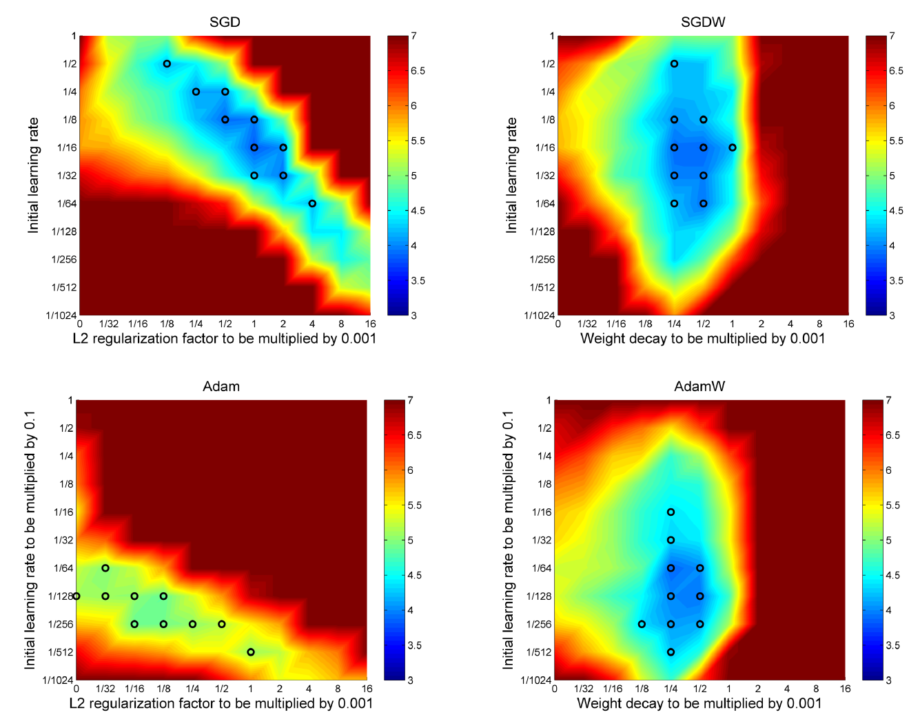
This figure is the core evidence of the whole paper. All four panels show the test error of a 26 2x64d ResNet trained on CIFAR-10 for 100 epochs; the vertical axis is the initial learning rate, the horizontal axis is the L2 coefficient or weight decay, bluer is better, and the black circles are the 10 best settings.
Top left, SGD with L2. The good region is a diagonal band. For example, the black circle in the top-left corner sits at and ; changing either one alone makes things worse, while changing both together might even make them better. This is exactly the of Proposition 1; when the learning rate changes, the best L2 coefficient changes with it. The authors suggest that SGD's reputation for being "sensitive to hyperparameters" may come partly from this coupling.
Top right, SGDW. The good region becomes a vertical strip, with most black circles at decay values between 1/4 and 1/2 (times 0.001), spanning five different learning rates. Even if the learning rate isn't tuned well, say stuck at 1/1024, tuning just the decay can still find a decent value.
Bottom left, Adam with L2. The best result is clearly worse than SGD's. Now look at where the black circles are. Settings with an L2 coefficient of 0 also make the top ten, so the best result with L2 is about the same as with none at all. In other words, L2 has almost no effect here, and the good region is diagonal as well.
Bottom right, AdamW. The good region is vertical, like SGDW's, with the black circles concentrated at decay values of 1/4 to 1/2; the best result is clearly better than Adam with L2, and on par with SGD and SGDW.
So this figure supports two things at once. After decoupling, the learning rate and weight decay can be tuned more or less separately; and once Adam switches to decoupled weight decay, it catches up with SGD on this task.
Better generalization, or just better training?
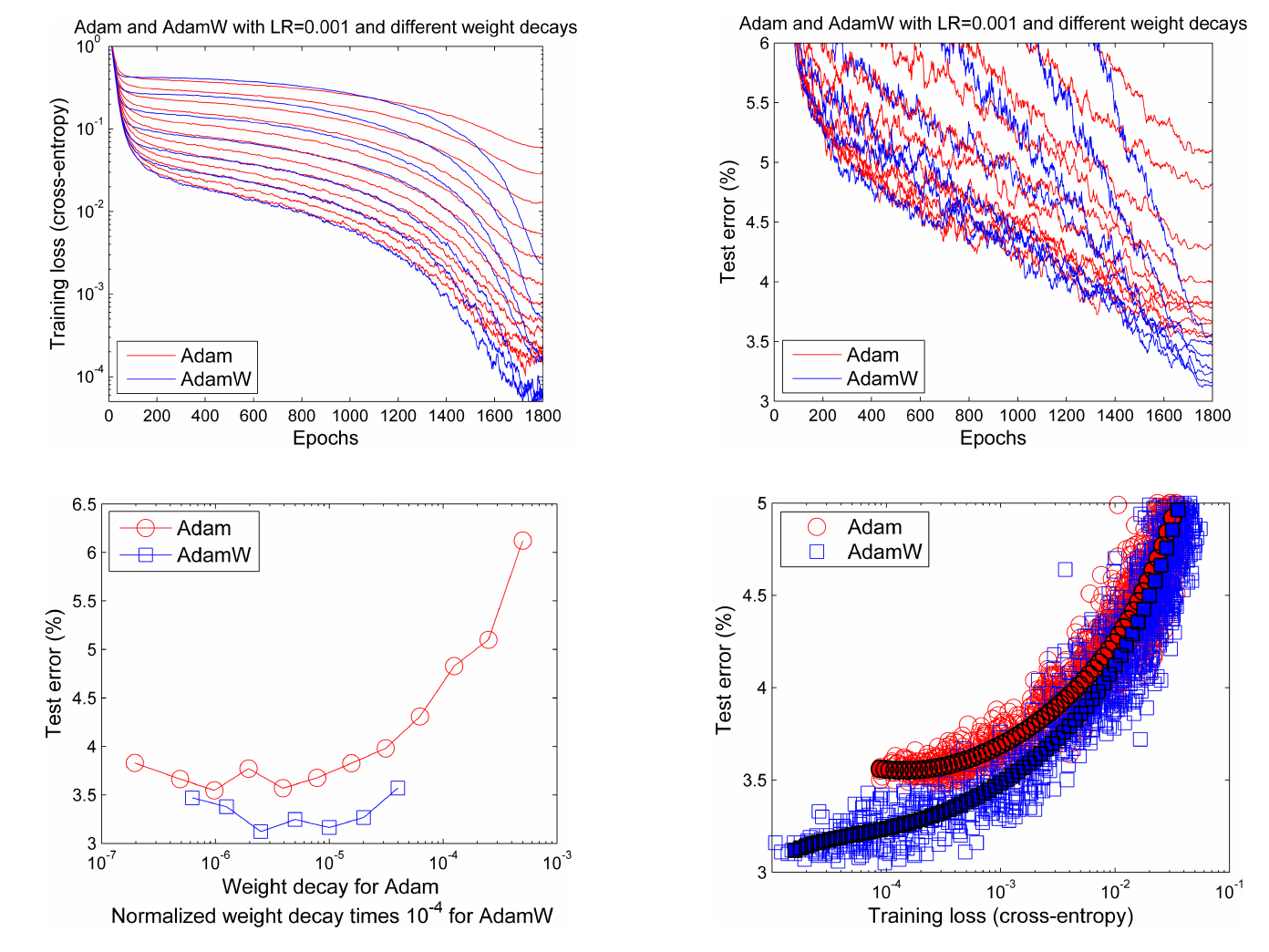
The heatmaps cover only 100 epochs of training. The authors then train the larger 2x96d for 1800 epochs, with the initial learning rate fixed at Adam's default of 0.001 (the schedule is still cosine annealing), trying 12 coefficients for Adam with L2 and 7 normalized decay values for AdamW.
In the learning curves on the top row, the two groups often overlap in the first half, while in the second half AdamW's training loss and test error are usually lower. The bottom left shows the final test error, with Adam with L2 at best about 3.55% and AdamW at best about 3.1%.
The bottom right plot answers the question in this section's title. The horizontal axis is training loss and the vertical axis is test error; if AdamW were simply driving the training loss lower, both groups of points should fall on the same curve. In fact, at the same training loss, the blue AdamW points have lower test error than the red Adam ones. From this the authors argue that AdamW not only trains better but also generalizes better. The results on ImageNet32x32 are the same.
Warm restarts and anytime results
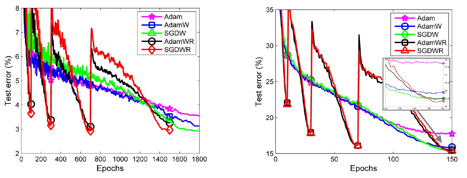
The last comparison adds warm restarts. The left panel is CIFAR-10. The two lines with an R jump up at every restart and then quickly fall to a low point; before the first restart (epoch 100), AdamWR has already reached about 4.0%, and the authors say this makes AdamW up to 10 times faster. This is what the paper calls "anytime" performance; stop halfway through training, and you still have a decent model.
The paper reports that at the default learning rate of 0.001, AdamW's test error is 15% lower than Adam's in relative terms, on both CIFAR-10 and ImageNet32x32, and that AdamWR achieves the same results while being usable at any time. Reading off the left panel, Adam on CIFAR-10 ends at about 3.6% and AdamW at about 3.1%. AdamWR closes most of the gap between Adam and SGDWR, and on ImageNet32x32 the two are on par.
Other tasks and limitations
Section 4.5 collects reports from other teams that used it. A team working on EEG classification provided a direct comparison under the same hyperparameters, with Deep4Net going from 71.37% to 73.68% and ResNet from 61.34% to 72.04%; OpenAI's 2018 GPT trained its Transformer with AdamW; and Zhang et al. compared SGD, Adam, and K-FAC on CIFAR and found that whenever L2 and weight decay are not equivalent, decoupled weight decay does better.
The limitations are also clear. The main experiments are all image classification, and the authors write in their conclusion that these results still need to be verified on more tasks, especially ones where regularization matters a lot. The square-root rule for normalized weight decay also rests on only a few experiments.
The learning rate gets multiplied back in
Back to that lr * weight_decay from earlier.
In the paper's AdamW, the decay is ; it follows only the schedule multiplier and is not multiplied by the base learning rate . PyTorch's AdamW does , where is the actual learning rate including the schedule, so the decay is . Optax's adamw does the same; its documentation states explicitly that the weight decay here is multiplied by the learning rate, consistent with PyTorch but different from the paper, which multiplies only by the schedule multiplier. Keras's AdamW likewise subtracts variable * wd * lr from the parameters.
Converting between them, the paper's equals PyTorch's lr × weight_decay. PyTorch's defaults are lr=1e-3 and weight_decay=1e-2, so each step decays by , equivalent to in the paper's formulation. The default values also differ from one library to the next, 0.01 in PyTorch, in Optax, and 0.004 in Keras, so when you move hyperparameters over, first check which formulation and which default you're dealing with.
This difference has a practical consequence. With PyTorch's formulation, changing the learning rate also changes the amount of decay, so the property from the heatmaps above, that the two hyperparameters can be tuned separately, no longer fully holds. In a February 2024 blog post, Fabian Schaipp demonstrated this on a synthetic ridge regression problem and recommended keeping lr × weight_decay constant when sweeping the learning rate with PyTorch's AdamW, so that doubling the learning rate halves the decay; he also mentioned that his experience training ViTs with timm was consistent with this, though he didn't release experiments for that part. Wang and Aitchison in 2024 looked at it from another angle, viewing the weights AdamW learns as an exponential moving average of recent updates, with a timescale of roughly steps. On ResNet, ViT, and NanoGPT, they found that the optimal timescale measured in epochs stays roughly fixed, so as the dataset grows, weight decay should shrink. This points in the same direction as the paper's normalized weight decay.
Some frameworks do keep the paper's formulation, for example MosaicML Composer's DecoupledAdamW, where the decay is multiplied only by "the current learning rate divided by the initial learning rate," that is, the schedule multiplier. Also, PyTorch's Adam has its own weight_decay, which is L2; to get AdamW's behavior inside Adam, you have to set decoupled_weight_decay=True separately.
What came after
AdamW went on to become standard equipment for training Transformers. LLaMA uses AdamW with and weight decay 0.1; OLMo 2 even excludes the embedding layer from weight decay; DeepSeek-V4 hands most of its parameters to Muon, but still uses AdamW for the weights of the embedding layer, the prediction head, and the normalization layers.
Conclusion
This paper proves that L2 regularization and weight decay are equivalent only in SGD, and even then only with the coefficient converted according to the learning rate; in Adam, the L2 gradient gets divided by , so weights with large past gradients are regularized less. Move the decay out of the gradient and apply it directly to the parameters, and you have AdamW. The CIFAR-10 heatmaps show that this lets the learning rate and weight decay be tuned more or less separately, and that Adam's best results catch up with SGD's; the 1800-epoch comparison shows that at the same training loss, AdamW has lower test error. The evidence comes mainly from ResNets on image classification, and the normalization rule rests on only a few experiments.
When you use it in practice, first check which AdamW you're using. In PyTorch, Optax, and Keras, the decay is the learning rate times weight_decay, while the paper's and Composer's versions multiply only by the schedule multiplier; when moving settings over from the paper or another framework, remember to convert. When sweeping the learning rate in PyTorch, you can hold lr × weight_decay fixed, and keep in mind that torch.optim.Adam(weight_decay=...) is L2, through and through.
The first version of the paper was titled "Fixing Weight Decay Regularization in Adam," and the fixed version went on to become standard equipment for large language models. It's just that the most widespread implementations multiplied the learning rate back into the decay term.