Original paper
Shampoo: Preconditioned Stochastic Tensor Optimization
- Publication
- ICML 2018Conference
- First submitted to arXiv
- arXiv:1802.09568
Cite this paper · BibTeX
The citation identifies the linked source version. It cites the original paper and its authors.
@misc{optimizersshampoo2018,
  title = {{Shampoo: Preconditioned Stochastic Tensor Optimization}},
  author = {Vineet Gupta and Tomer Koren and Yoram Singer},
  year = {2018},
  eprint = {1802.09568},
  archivePrefix = {arXiv},
  url = {https://arxiv.org/abs/1802.09568}
}
The paper's name is tucked away in a footnote on page 2: “We call it Shampoo because it has to do with preconditioning.”
Conditioner is what goes on your hair, so pre-conditioning is whatever comes before it, which is obviously shampoo. The acknowledgments also give special thanks to Roy Frostig for coming up with the name.
Jokes aside, the paper tackles a very practical headache. An optimizer that wants to see how parameters pull on one another has to maintain a matrix the size of the parameter count squared. Vineet Gupta and Tomer Koren of Google Brain and Yoram Singer of Princeton wanted a way to avoid actually storing that matrix.
Defining the problem
What preconditioning does
In the plainest gradient descent, every parameter moves against its gradient with the same learning rate. A preconditioned method first multiplies the gradient by a matrix before taking the step:
If is diagonal, the effect is to scale each parameter's step separately; Adam and AdaGrad both belong here. If is a full matrix, it can also “turn” the gradient. When the loss landscape is a long, narrow valley running diagonally, two parameters have to move together to follow the valley floor. A diagonal matrix can only scale the two coordinate axes separately; it takes a full matrix to rotate that slanted valley straight.
Full-matrix AdaGrad is too big
AdaGrad has a full-matrix version whose preconditioner is the square root of the accumulated outer products of the gradients:
Its theoretical properties are better than the diagonal version's, but nobody can afford it. Take a fully connected layer. Flattened, it has million parameters, so is , about entries, which takes more than 4 TB in single precision; on top of that, every step needs its square root and inverse, at a cost of .
There were a few ways out at the time. Diagonal approximations are cheap but throw away every correlation between parameters. Sketching and other estimation methods the authors judge “seldom practical at large scale.” K-FAC also uses a Kronecker factorization, but what it approximates is the Fisher matrix; it has to sample from the model's predictive distribution and relies on the backpropagation structure of feed-forward networks, so a new architecture means a new derivation.
Neural network parameters are matrices and tensors to begin with. A fully connected layer is , and a convolution kernel has four dimensions. The question this paper asks is whether we can keep that shape and approximate the huge preconditioner with a few small matrices.
Solving the problem
One on each side
In the matrix case, Shampoo keeps two preconditioners for an weight matrix, an one on the left and an one on the right (Algorithm 1):
They start at and . accumulates correlations between rows, which for a fully connected layer means between output units; accumulates correlations between columns, that is, between input features. In the update, the gradient is multiplied once from the left and once from the right.
For the same layer, and together hold million entries, 8 MB in single precision. Memory drops from to , and the cost of computing the matrix powers drops from to .
These two small matrices are really one big matrix in disguise. By the Kronecker-product identity in the paper's Lemma 4, flattening gives times the flattened gradient. So Shampoo is effectively using an preconditioner ; it just never assembles that matrix.
In code, the update for one matrix parameter is only a few lines:
import torch

def matrix_power(A, p):
    """p-th power of a symmetric positive-definite matrix: eigendecompose, then raise only the eigenvalues to p"""
    lam, Q = torch.linalg.eigh(A)
    return Q @ torch.diag(lam ** p) @ Q.T

class ShampooMatrix:
    """Algorithm 1: Shampoo for one m×n weight matrix"""
    def __init__(self, m, n, lr, eps=1e-4):
        self.L = eps * torch.eye(m)   # L_0 = εI_m
        self.R = eps * torch.eye(n)   # R_0 = εI_n
        self.lr = lr

    @torch.no_grad()
    def step(self, W, G):
        self.L += G @ G.T             # accumulate the m×m left statistic
        self.R += G.T @ G             # accumulate the n×n right statistic
        W -= self.lr * matrix_power(self.L, -0.25) @ G @ matrix_power(self.R, -0.25)
The paper's own implementation is in TensorFlow and computes the matrix powers with an SVD; the approach is the same.
Why 1/4
AdaGrad takes a square root, so shouldn't the exponent be ? Shampoo uses instead, once on each side.
The answer is in Lemma 8. Assuming every gradient matrix has rank at most , the authors prove
The left side is the full AdaGrad statistic. The proof has two steps. It first shows and separately, an upper bound from each side; then, using the monotonicity of the matrix geometric mean, it raises each bound to the power and multiplies them. That's where the first comes from.
AdaGrad's preconditioner takes one more square root of the statistic. The square root preserves order on positive semidefinite matrices, so taking the power of both sides gives
So , with one half from the geometric mean and the other from AdaGrad's square root. Shampoo's is a Kronecker-structured matrix sitting on top of the full AdaGrad preconditioner. The authors point out that the small eigenvalues of the full-matrix preconditioner, the ones that matter most for preconditioning, do not vanish under this approximation.
The paper also offers an intuition. This exponent makes the overall step size decay as , a rate common in stochastic optimization. When gradient magnitudes are steady, and grow roughly linearly with the step count ; and each contribute , which together make exactly .
This is a by-product of the upper bound in the proof. Later implementations made the exponent tunable and often switch to ; we'll come back to that in the discussion.
The tensor version
Convolution kernels are four-dimensional. The general form of Shampoo (Algorithm 2) keeps an preconditioner for each dimension of the tensor, whose statistic is the matrix obtained by contracting the gradient over all the other dimensions. The update multiplies by one dimension at a time, where is the tensor's order. For a matrix, , which brings back .
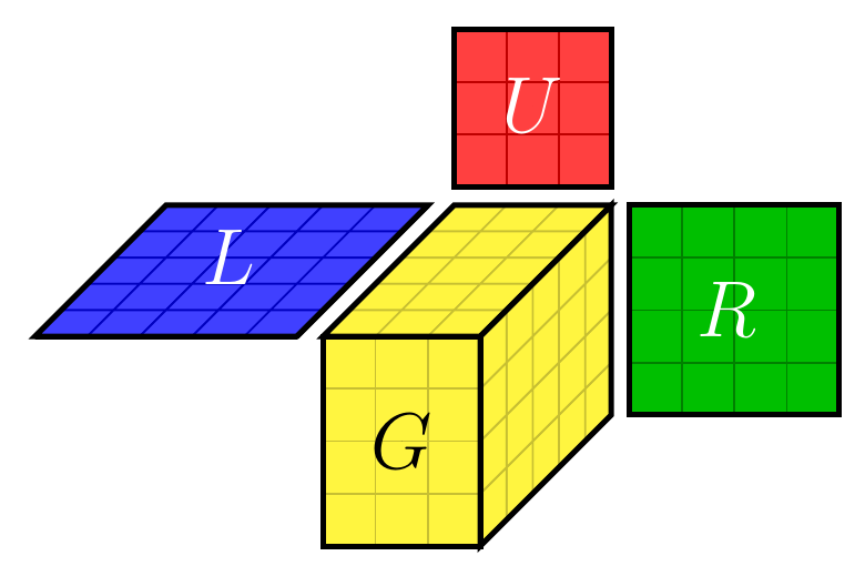
Take the largest convolution kernel in the paper's CIFAR-100 experiment, . It has 589,824 parameters, and the full AdaGrad preconditioner would have about entries. Shampoo needs only four matrices, entries, with an exponent of .
The convergence guarantee and its conditions
The theory is proved in the online convex optimization framework (Theorem 7). With gradient rank at most , the regret is bounded by
is the largest distance between and the optimum over the iterations. If the gradients' spectral norm is at most 1, each trace grows as and the total regret is , already the best possible rate in online convex optimization. The tensor version (Theorem 10) works the same way, with replaced by the geometric mean of the per-dimension ranks.
Read the conditions carefully. The loss must be convex. can grow with , and keeping it bounded requires projecting back into a ball at every step, using the norm induced by . That projection is expensive, so the authors leave it out of the algorithm and accept a “slightly looser” bound. Deep networks are not convex; this proof is where the algorithm comes from and what motivated it, while the experiments are the evidence for how it does on neural networks.
Compromises in practice
The implementation makes two trade-offs. Each parameter tensor is handled on its own, so the overall preconditioner is block-diagonal and correlations between layers are simply ignored. When a dimension is too large (the threshold in the experiments is about 1200), that dimension automatically switches to the diagonal version (Algorithm 3 in Appendix A) and stores only the diagonal entries. On top of that, the experiments add two heuristics: the matrix roots are recomputed only every 20 to 100 steps, and the gradient gets momentum with a coefficient of 0.9. The authors say the former has “almost no impact” on accuracy.
Discussion
The experiments are small
Every experiment uses a batch size of 128, and the preconditioners are updated with the batch-averaged gradient. Image classification uses a 32-layer ResNet with 2.4M parameters and a small Inception with 1.65M parameters on CIFAR-10, plus a 55-layer ResNet without BatchNorm with 13.5M parameters on CIFAR-100; each optimizer sweeps 10 learning rates between 0.01 and 10. For this part the paper plots only training-loss curves, with no table comparing test accuracy.
The language model is a 9.8M-parameter Attention model on LM1B, whose largest tensor is .
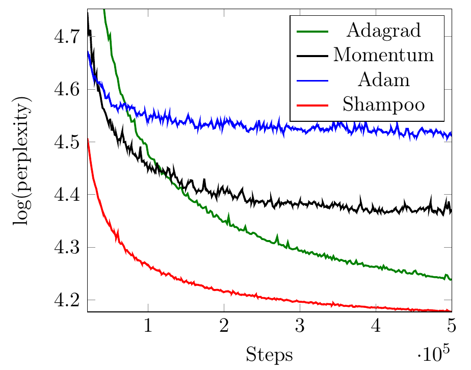
The red line is lowest from its very first point and sits around 4.18 at 500k steps; green AdaGrad is around 4.24, black Momentum around 4.37, and blue Adam levels off near 4.5 early on.
The comparison in this figure isn't symmetric. Shampoo simply uses the default learning rate , while for the other methods the authors “explored various different settings,” without listing which values Adam was swept over. Adam trails AdaGrad by a wide margin on this Attention model. Our reading is that this sits poorly with the later experience of Transformers being trained almost universally with Adam, and the gap most likely comes from uneven tuning; factor that in when reading this figure.
How much more each step costs
The paper answers “won't the matrix operations be too slow?” with a table of steps per second (Tesla K40, batch 128):
| Experiment | SGD | Shampoo | Ratio |
|---|---|---|---|
| ResNet-32 (C10) | 2.184 | 2.151 | 98% |
| Inception (C10) | 3.638 | 3.506 | 96% |
| ResNet-55 (C100) | 1.210 | 1.249 | 103% |
| Attention (LM1B) | 4.919 | 3.509 | 71% |
Compiled from Table 1 of the paper; the ratios are our calculation. Adam and AdaGrad are close to SGD and omitted.
On convolutional networks there's almost no difference, and ResNet-55 is even slightly faster than SGD. On LM1B, steps per second drop to 71% of SGD's, and the paper doesn't analyze why; the model's largest tensor is , and with the roughly 1200 threshold used in the experiments, the dimension of 2000 would switch to the diagonal version. These numbers were measured on models of only a few million parameters, with roots computed every 20 to 100 steps.
Shampoo after this paper
The 2018 original was a long way from large-scale training. The two versions that followed were mostly engineering.
Distributed Shampoo, Anil et al. (2020). The authors include all three from the original paper, and the paper is titled “Scalable Second Order Optimization for Deep Learning.” They found that in real models and have enormous condition numbers, so the matrix roots have to be computed in double precision, which is expensive on TPUs. The changes include:
- The accelerators only accumulate statistics each step; every steps, the inverse -th roots are computed asynchronously on the host CPUs, spread across all cores, without blocking the training loop;
- Coupled Newton iterations replace the SVD for the inverse roots, with warm starts;
- Layers with dimensions in the millions, such as embeddings and softmax, are preconditioned on one side only, and large fully connected layers are split into blocks preconditioned separately;
- The preconditioners are updated only every few hundred steps;
- Grafting: the direction comes from Shampoo and the step size from a tuned first-order method (for example, diagonal AdaGrad), grafted layer by layer;
- The exponent becomes a tunable hyperparameter, and the statistics use an exponential moving average.
On WMT'14 English-to-French, the Transformer needed half as many steps and 45% less wall-clock time (from about 12 hours down to 6.7 hours).
The PyTorch version, Shi et al. (2023). A Meta team rewrote it for data-parallel training on GPUs. Each worker preconditions only some of the parameter blocks, and the resulting directions are gathered with AllGather, so per-step wall-clock time is at most 10% more than with diagonal methods. The matrix roots switch to torch.linalg.eigh, and they found single precision is usually enough. Small dimensions are merged and large ones split into blocks, with a block size cap of 2048 in the ImageNet experiments; grafting, bias correction, decoupled weight decay and Nesterov are all included. On ResNet-50 for ImageNet, Shampoo reaches in 60 epochs the validation accuracy SGD-Nesterov reaches in 90, finishing 1.35 times faster in total wall-clock time.
AlgoPerf 2024. In August 2024, MLCommons announced the results of the first AlgoPerf training algorithms competition. The winner of the external tuning track was this PyTorch Distributed Shampoo, with a score of 0.78, about 28% faster than the NAdamW baseline on average. The post-competition analysis paper has the more interesting details. Of the eight workloads, it was fastest on only two, Criteo 1TB and ViT; on WMT it took more than twice as long as the fastest submission; and on ResNet it failed to reach the target reliably within the time budget. It won by being consistently decent on almost everything.
The Gemini 1.5 technical report from the same year also says that 1.5 Flash “is trained with higher-order preconditioned methods,” citing AdaGrad among other works without naming the method.
1/4 or 1/2
The exponent question was eventually settled. Anil et al. note in their appendix that treating the exponent as a hyperparameter sometimes works better, and their autoencoder experiments use ; Shi et al.'s implementation suggests that for networks dominated by fully connected layers you can override the exponent to , again , or multiply the original exponent by 1.82. Morwani et al. (2024) explained why. is exactly the result of one step of power iteration toward the best Kronecker approximation of the full AdaGrad statistic, and it lands very close to that best approximation. Since is itself approximating , mimicking AdaGrad's power means taking on each side. Looking back from Morwani et al. (2024), we would sum up the original paper's as an exponent produced by a bound that isn't tight enough.
The wasn't wasted, though. Drop the accumulation and look only at the current step's gradient :
Every singular value is squashed to 1, which is exactly Muon's orthogonalized update. On Shampoo's first step, the statistics hold a single gradient, so with a small ε the direction it moves in is . Taking one step with the code above on a random gradient, the result differs from only by the offset ε introduces, mostly on the order of . Keller Jordan's December 2024 post introducing Muon also notes that Shampoo without accumulation, plus momentum, is Muon; the difference is that Shampoo computes inverse fourth roots, while Muon approximates them cheaply with Newton–Schulz iterations.
Conclusion
Shampoo approximates full-matrix AdaGrad's unstorable preconditioner with the Kronecker product of two small matrices, cutting memory from to , and proves regret in the convex setting. The paper's experiments stop at around ten million parameters and mainly show that each step isn't much slower.
If you want to try it today, go straight to Meta's Distributed Shampoo. Start tuning from Adam grafting, an exponent of and preconditioner updates every few dozen steps, and first measure how much the largest dimension in your model slows each step down. Keep the original code for understanding the algorithm.
Page 12 of the paper says, “We plan to implement Shampoo in PyTorch in the near future.” The version that went on to win AlgoPerf was indeed a PyTorch one, written by a Meta team five years later.