Original paper
SGDR: Stochastic Gradient Descent with Warm Restarts
- Publication
- ICLR 2017Conference
- First submitted to arXiv
- arXiv:1608.03983
Cite this paper · BibTeX
The citation identifies the linked source version. It cites the original paper and its authors.
@misc{optimizerssgdr2016,
  title = {{SGDR: Stochastic Gradient Descent with Warm Restarts}},
  author = {Ilya Loshchilov and Frank Hutter},
  year = {2016},
  eprint = {1608.03983},
  archivePrefix = {arXiv},
  url = {https://arxiv.org/abs/1608.03983}
}
Open PyTorch's torch.optim.lr_scheduler, and the documentation of two schedulers points to the same paper.
One is CosineAnnealingWarmRestarts, whose name already spells out where it comes from. The other is CosineAnnealingLR, whose documentation cites the same paper but makes a point of adding that, although SGDR has periodic restarts, this implementation does cosine annealing without restarts.
For a paper with "restarts" in its title, the part that survived into the training setups of large models is mostly the half without restarts. Let's go back to the beginning and see what Ilya Loshchilov and Frank Hutter actually proposed in 2016, and what problem restarts were originally meant to solve.
If you haven't heard of these two authors, here is a bit of background. They were at the University of Freiburg in Germany at the time. Hutter's main research focus is hyperparameter optimization and AutoML; Loshchilov had done a good deal of earlier work on the evolution strategy CMA-ES, and when Section 2 of the paper reviews restart strategies, his own 2012 work is among those cited. In gradient-free optimization, "run for a while, then start over completely" is an old trick for dealing with multimodal functions, and a common practice is to double the population size at every restart. This paper brought the habit of restarting into SGD.
Defining the problem
In 2016, the mainstream way to train networks like ResNet was SGD with momentum, which is the paper's Eqs. (3) and (4):
The authors say in the introduction that the hardest remaining parts of training this way are how to schedule the learning rate and how much weight decay to use. The baseline used in this paper, Wide ResNet (WRN), starts the learning rate at 0.1 and multiplies it by 0.2 at epochs 60, 120, and 160, training for 200 epochs in total.
This kind of step schedule has two drawbacks. First, where to drop and by how much are both hyperparameters to tune. Second, the model only gets good after the learning rate has come down; if you have to stop at epoch 100, the model you're holding is still stuck in the high-learning-rate phase, with a large error. The authors describe the latter with the term anytime performance, meaning that whenever you stop, you have a good enough model in hand.
The goal of this paper is to improve SGD's anytime performance. How should the learning rate be scheduled so that training can be stopped at any time, and still end up no worse than a well-tuned step schedule?
Solving the problem
Warm restarts
The authors' approach is to simulate a fresh start of SGD every epochs. This restart doesn't retrain from scratch. The parameters are kept exactly as they are and used as the new starting point; only the learning rate is pulled back up and then allowed to come down again. The paper also notes that how far the learning rate is raised determines how much of the previously accumulated information (such as momentum) is kept.
Cosine annealing
Within the -th run, the learning rate decreases batch by batch according to Eq. (5):
is the number of epochs run since the last restart. It is updated at every batch, so it can take fractional values like 0.1 or 0.2. Let's plug in a few points:
- , , and the learning rate is .
- , , and the learning rate is exactly halfway between the two ends.
- , , and the learning rate drops to .
So this curve falls slowly at first, is close to a straight line in the middle, and slows down again near the end, lingering at a low learning rate for a while. In the CIFAR experiments, and are fixed at 0.05 and 0 for every run. The authors mention that lowering these two values at each restart might help, but they didn't do it, to keep the number of hyperparameters down.
and
The length of each period is set by two numbers. is the length of the first run, and after each restart the period is multiplied by . Here is the calculation for the setting that appears most often in the paper, and :
| Run | Period length | Ends at epoch |
|---|---|---|
| 1 | 10 | 10 |
| 2 | 20 | 30 |
| 3 | 40 | 70 |
| 4 | 80 | 150 |
| 5 | 160 | 310 |
Within a budget of 200 epochs, only the first four runs finish; the fifth ends halfway through. With and instead, the restarts fall at epochs 1, 3, 7, 15, 31, 63, and 127.
The point of doubling the period is to get a usable model quickly with very short periods first, then trade increasingly long periods for better results, which is the same idea as the evolution strategies mentioned earlier doubling the population at every restart. Another setting is , restarting every epochs; with , the whole of training is a single cosine with no restarts at all. This line will become very important later on.
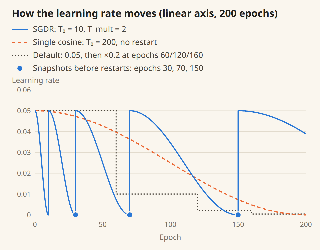
The paper plots these schedules on a log axis, and the authors themselves acknowledge that the log axis hides the cosine shape, so here we redraw them on a linear axis. The blue line jumps right back to 0.05 every time it hits 0, while the orange dashed line comes down slowly from 0.05 all the way to 0.
Which model do you hand over?
When the learning rate is suddenly raised, the model temporarily gets worse, so SGDR doesn't necessarily hand over the parameters from the last step. Before the first restart, the recommended solution is simply the latest ; after that, it is the end of the most recently completed period, the model at the point where the learning rate has just reached . In the table above, at epoch 200 SGDR hands over the model from epoch 150. The authors stress that this rule doesn't need a separate validation split to pick the model.
Why restart
Section 2 reviews two lines of work. Gradient-free optimization uses restarts to deal with multimodal functions; gradient-based optimization mostly uses restarts to speed up convergence. For example, O'Donoghue and Candès (2012) found that Nesterov's accelerated method oscillates periodically when momentum overshoots, so they restart whenever the objective increases, or when the momentum direction forms an obtuse angle with the negative gradient.
The stochastic-gradient case is different. The loss and gradient of a single batch are too noisy for these criteria to carry over directly; they would first have to be averaged (once per epoch, for example). The authors chose the simplest version, restarting on a fixed schedule. In the discussion they are also quite cautious, saying the main purpose of SGDR is to improve anytime performance, and that they do not claim to have observed any effect related to multimodality.
Discussion
Experimental setup
The main experiments train WRN-28-10 (28 layers, with 10 times as many filters per layer as the original ResNet, about 36.5 million parameters) on CIFAR-10 and CIFAR-100. The authors first reproduce the settings of the original WRN paper: momentum 0.9, weight decay 0.0005, batch size 128, 200 epochs, with data augmentation by horizontal flips and random crops after 4-pixel reflection padding. It differs from the original setup in only two places, subtracting only the per-pixel mean without ZCA whitening, and using the plain momentum of Eqs. (3) and (4) instead of Nesterov momentum.
Single models
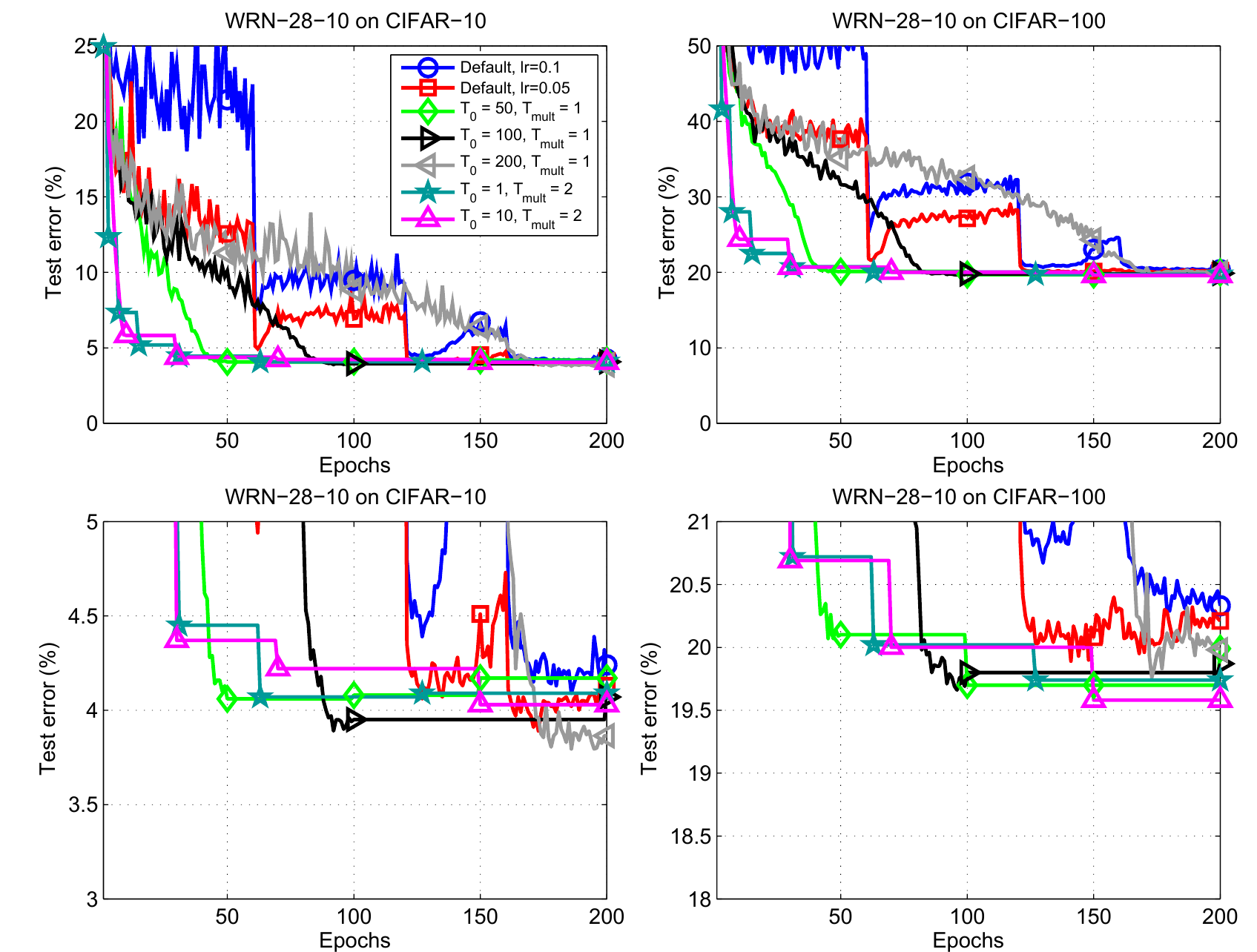
Start with the top row. The blue and red lines are the default schedule. Before the learning-rate drop at epoch 60, their CIFAR-10 test error stays above 12%, and even after one drop it is still between 7% and 10%; on CIFAR-100, the red line even climbs between the two learning-rate drops. The SGDR lines plot the recommended solutions, which is why they look like staircases; the period-doubling green stars () and magenta triangles () fall into the low-error region within a few dozen epochs. The bottom row zooms in on the same results, showing which lines end higher or lower over the last few epochs.
The authors conclude that SGDR reaches test errors of about 4% on CIFAR-10 and about 20% on CIFAR-100 with 2 to 4 times fewer epochs. The final numbers are summarized below:
| WRN-28-10 schedule | CIFAR-10 | CIFAR-100 |
|---|---|---|
| Default, η₀ = 0.1 | 4.24 | 20.33 |
| Default, η₀ = 0.05 | 4.13 | 20.21 |
| T₀ = 50, T_mult = 1 | 4.17 | 19.99 |
| T₀ = 100, T_mult = 1 | 4.07 | 19.87 |
| T₀ = 200, T_mult = 1 | 3.86 | 19.98 |
| T₀ = 1, T_mult = 2 | 4.09 | 19.74 |
| T₀ = 10, T_mult = 2 | 4.03 | 19.58 |
Compiled from Table 1 of the paper; test error (%), median of five runs.
Two things to watch for when reading this table. First, most of the differences are only a few tenths of a percentage point, each setting was run only five times, and the authors note in the table caption that the bold numbers just mark the better results, with no statistical test. Second, the best single model on CIFAR-10, at 3.86%, comes from , , a single complete cosine with no restarts at all. The authors take this as a sign that WRN's original step schedule may not be the best choice; but this setting also has the worst anytime performance, catching up only in the last few epochs.
The authors spent the time saved on training the wider WRN-28-20 (145.8 million parameters, about 3 to 4 times the compute). CIFAR-10 improved by about 0.25 percentage points and CIFAR-100 by 0.5 to 1 percentage point, with , reaching 3.74% and 18.70%. Looking at just the first 50 epochs, WRN-28-20 paired with , before any restart, was already below 19% on CIFAR-100, while WRN-28-10 never did better than 19.5% with any schedule.
The training curves in the appendix add one more observation. Up to about epoch 120, SGDR's training loss falls faster than the default schedule's; after that, the default schedule starts to overfit, with the test loss climbing, while SGDR overfits only slightly.
Free snapshot ensembles
After the first arXiv version of SGDR came out, Huang et al.'s Snapshot Ensembles used its periods to build ensembles. Just before each restart, the learning rate has just bottomed out and the model has settled at a good position; save these snapshots, and you can assemble a set of models at no extra training cost. The final version of this paper goes back and checks whether the idea holds up on WRN.
The procedure is to train WRN-28-10 with SGDR at , and save snapshots at epochs 30, 70, and 150, the three blue dots on the schedule chart. At inference time, the softmax output probabilities of the snapshots are averaged with equal weights.
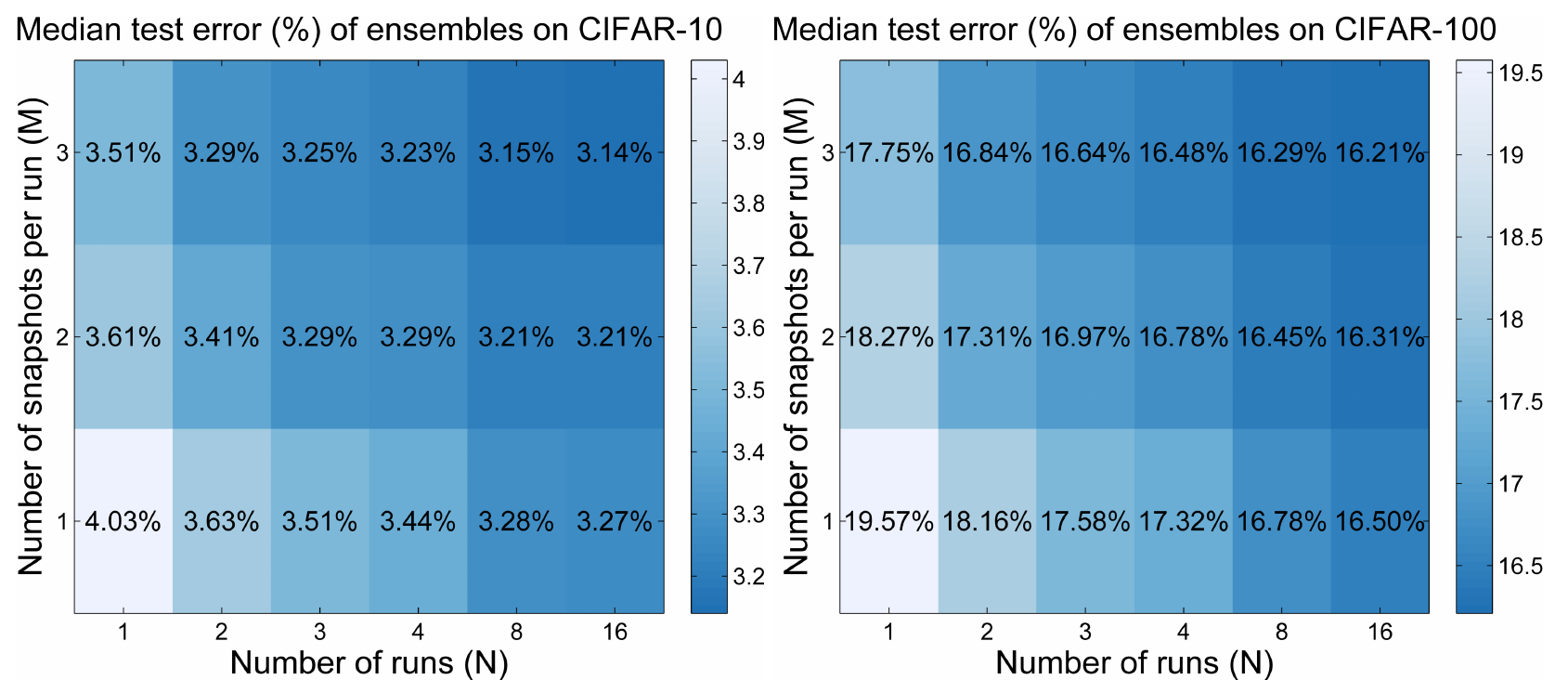
The horizontal axis is how many independent training runs (), and the vertical axis is how many snapshots are taken from each run (). The bottom-left corner is a single model, 4.03% on CIFAR-10 and 19.57% on CIFAR-100 (the median of 16 runs). Going up to , the three snapshots from a single run already bring this down to 3.51% and 17.75%. Getting a similar effect from independent training takes runs (3.51% and 17.58%), so in this setting the snapshots cut the training needed roughly threefold.
Where the snapshots come from matters too. Ensembling only the models from the last three epochs (148, 149, 150) gives the same result as using only the model from epoch 150, with no improvement. The snapshots taken before restarts help because they come from different periods, so their predictions differ from one another.
The two approaches can be stacked. Three training runs with 3 snapshots each bring the error down to 3.25% and 16.64%; 16 runs with 3 snapshots each give the 3.14% and 16.21% from the abstract, the paper's claimed state of the art on CIFAR at the time, though that is an ensemble of 48 models. The two datasets don't follow quite the same trend either. On CIFAR-10, 9 snapshots (, ) at 3.25% are already on par with 16 independent models at 3.27%; on CIFAR-100, 16 independent models at 16.50% are still slightly better than 9 snapshots at 16.64%.
EEG and downsampled ImageNet
To show that the method isn't limited to CIFAR, the authors ran two more sets of experiments.
The first uses electroencephalography (EEG) data, from 14 subjects with about 1,000 trials each, where the task is to classify actual movements of the left hand, right hand, and feet, using the convolutional network designed by Schirrmeister et al. The baseline schedule has to fix the total number of epochs in advance (from 30 to 480) and then cut the learning rate by a factor of 10 at fixed proportional points; the larger the budget, the better the result. SGDR doesn't need the budget decided in advance; its final performance is about the same as the baseline, and its performance along the way is better. Ensembling snapshots also works. Against a median reference error of about 9%, taking snapshots from a single training run lowers it by another 1 to 2 percentage points, and combining snapshots from two learning-rate settings lowers it by 2 to 3 percentage points.
The second uses a downsampled ImageNet the authors made themselves, with the same 1,000 classes and the same images as the original, only shrunk to 32 × 32 with box downsampling (this dataset was later published separately in 2017). Each image has two orders of magnitude fewer pixels on average, so it is harder than the original ImageNet; with more classes, and objects that often occupy only a small part of the frame, it is also harder than CIFAR. On WRN-28-10, they compare the default schedule with two SGDR settings, each with 4 initial learning rates (0.05, 0.025, 0.01, 0.005). SGDR with , , reaches top-1 and top-5 errors of 39.24% and 17.17%, comparable to AlexNet's 40.7% and 18.2% on full-resolution ImageNet. This experiment ran for only about 40 epochs, and the authors themselves call it a preliminary result; the comparison with AlexNet crosses resolutions and models, so it only serves as a rough point of reference.
The authors' reading of these results is that the choice of initial learning rate matters a lot, and since every SGDR period sweeps all the way from the initial value down to 0, it effectively tries out a whole range of learning rates, softening the damage from picking the wrong initial value.
Are restarts really the point?
The best single models on CIFAR-10, WRN-28-10 at 3.86% and WRN-28-20 at 3.66%, both come from without restarts. The authors also write in the discussion that even without any restarts, the aggressive schedule of Eq. (5) is quite competitive with the default schedule, and it needs only two hyperparameters, the initial learning rate and the total number of epochs.
Later research made this clearer. Gotmare et al. (ICLR 2019) used mode connectivity to analyze SGDR's trajectory, training VGG-16 on CIFAR-10 with the same , schedule. Between the models at epochs 30 and 150, and at epochs 70 and 150, the training loss along the connecting path is indeed higher than at the two ends, meaning the parameters crossed a barrier after the restart; but the models at epochs 70 and 150 are neither local minima nor, by the look of it, in different basins, so the "escaping local minima" story may be oversimplified. In a footnote they add that what consistently worked well in their experiments was a single cosine (or linear) decay over the whole budget, and they speculate that the decay is what really does the work, with restarts contributing less.
That is also how people use it in practice. fast.ai promoted SGDR in its 2017 course through cycle_len and cycle_mult; by fastai v1 at the end of 2018, a maintainer replied on the forums that this API no longer worked and that the default had changed to 1cycle. Later large-scale training mostly runs just a single cosine period:
- Bag of Tricks (He et al., 2018) uses a "simplified version" on ImageNet, with the learning rate following a cosine from its initial value all the way down to 0 (warmup counted separately).
- GPT-3 uses a cosine to bring the learning rate down to 10% of its original value over 260 billion tokens, and then holds it at 10%; the first 375 million tokens are a linear warmup.
- LLaMA's cosine schedule sets the final learning rate to 10% of the maximum, with 2,000 warmup steps.
Run only a single period, though, and you need to know the total number of steps in advance, which brings back the very problem SGDR set out to address. The Chinchilla appendix quantified the cost, finding that setting the cosine period more than 25% longer than the actual number of training steps makes the model noticeably worse. The later WSD (a three-phase schedule of warmup, stable, and decay), WSM, and Schedule-Free all deal with exactly this.
Conclusion
SGDR writes the learning-rate schedule as a single formula. Each period descends along a cosine from to , the period lengths are set by and , and when a period ends, the learning rate is pulled back up to start again. On CIFAR, it reaches errors comparable to a step schedule with 2 to 4 times fewer epochs, and the snapshots taken before restarts can form an ensemble for free; meanwhile, the best single model on CIFAR-10 comes from a single cosine without restarts.
If you know how long you'll be training in total, the simplest choice is one complete cosine period, with equal to the total number of steps and warmup added in front if needed; CosineAnnealingLR is exactly that version. Only when you want snapshot ensembles, or genuinely don't know your budget, is it worth bringing out CosineAnnealingWarmRestarts; and in that case, remember to follow the paper's rule and hand over the model from the end of a period, not from the last step.
The names of these two PyTorch schedulers have already made the choice for you. If you're not planning to restart, just pick the one with the shorter name.