Original paper
DeepSeek-V4: Towards Highly Efficient Million-Token Context Intelligence
- Publication
- Publication venue not yet verified
- First submitted to arXiv
- arXiv:2606.19348
Cite this paper · BibTeX
The citation identifies the linked source version. It cites the original paper and its authors.
@misc{deepseekdeepseekv42026,
  title = {{DeepSeek-V4: Towards Highly Efficient Million-Token Context Intelligence}},
  author = {DeepSeek-AI and Anyi Xu and Bangcai Lin and Bing Xue and Bingxuan Wang and Bingzheng Xu and Bochao Wu and Bowei Zhang and Chaofan Lin and Chen Dong and Chenchen Ling and Chengda Lu and Chenggang Zhao and Chengqi Deng and Chengyu Hou and Chenhao Xu and Chenze Shao and Chong Ruan and Conner Sun and Damai Dai and Daya Guo and Dejian Yang and Deli Chen and Donghao Li and Dongjie Ji and Erhang Li and Fang Wei and Fangyun Lin and Fangzhou Yuan and Feiyu Xia and Fucong Dai and Guangbo Hao and Guanting Chen and Guoai Cao and Guolai Meng and Guowei Li and Han Yu and Han Zhang and Hanwei Xu and Hao Li and Haofen Liang and Haoling Zhang and Haoming Luo and Haoran Wei and Haotian Yuan and Haowei Zhang and Haowen Luo and Haoyu Chen and Haozhe Ji and Hengqing Zhang and Honghui Ding and Hongxuan Tang and Huanqi Cao and Huazuo Gao and Hui Qu and Hui Zeng and J Yang and JQ Zhu and Jia Luo and Jia Song and Jia Yu and Jialiang Huang and Jialu Cai and Jian Liang and Jiangting Zhou and Jiasheng Ye and Jiashi Li and Jiaxin Xu and Jiewen Hu and Jieyu Yang and Jin Chen and Jin Yan and Jingchang Chen and Jingli Zhou and Jingting Xiang and Jingyang Yuan and Jingyuan Cheng and Jingzi Zhou and Jinhua Zhu and Jiping Yu and Joseph Sun and Jun Ran and Junguang Jiang and Junjie Qiu and Junlong Li and Junmin Zheng and Junxiao Song and Kai Dong and Kaige Gao and Kang Guan and Kexing Zhou and Kezhao Huang and Kuai Yu and Lean Wang and Lecong Zhang and Lei Wang and Leyi Xia and Li Zhang and Liang Zhao and Lihua Guo and Lingxiao Luo and Linwang Ma and Linyan Zhu and Litong Wang and Liyu Cai and Liyue Zhang and Longhao Chen and MS Di and MY Xu and Max Mei and Miaojun Wang and Mingchuan Zhang and Minghua Zhang and Minghui Tang and Mingming Li and Mingxu Zhou and Minmin Han and Ning Wang and Panpan Huang and Panpan Wang and Peixin Cong and Peiyi Wang and Peng Zhang and Qiancheng Wang and Qihao Zhu and Qingyang Li and Qinyu Chen and Qiushi Du and Qiwei Jiang and Rui Tian and Ruifan Xu and Ruijie Lu and Ruiling Xu and Ruiqi Ge and Ruisong Zhang and Ruizhe Pan and Runji Wang and Runqian Chen and Runqiu Yin and Runxin Xu and Ruomeng Shen and Ruoyu Zhang and Ruyi Chen and SH Liu and Shanghao Lu and Shangmian Sun and Shangyan Zhou and Shanhuang Chen and Shaofei Cai and Shaoheng Nie and Shaoqing Wu and Shaoyuan Chen and Shengding Hu and Shengyu Liu and Shiqiang Hu and Shirong Ma and Shiyu Wang and Shuiping Yu and Shunfeng Zhou and Shuting Pan and Shuying Yu and Songyang Zhou and Tao Ni and Tao Yun and Tian Jin and Tian Pei and Tian Ye and Tianle Lin and Tianran Ji and Tianyi Cui and Tianyuan Yue and Tingting Yu and Tun Wang and W Zhang and WL Xiao and Wangding Zeng and Wei An and Weilin Zhao and Wen Liu and Wenfeng Liang and Wenjie Pang and Wenjing Luo and Wenjing Yao and Wenjun Gao and Wenkai Yang and Wenlve Huang and Wenqing Hou and Wentao Zhang and Wenting Ma and Xi Gao and Xiang He and Xiangwen Wang and Xianzu Wang and Xiao Bi and Xiaodong Liu and Xiaohan Wang and Xiaokang Chen and Xiaokang Zhang and Xiaotao Nie and Xiaowen Sun and Xiaoxiang Wang and Xin Cheng and Xin Liu and Xin Xie and Xingchao Liu and Xingchen Liu and Xingkai Yu and Xingyou Li and Xinyu Yang and Xinyu Zhang and Xu Chen and Xuanyu Wang and Xuecheng Su and Xueyin Chen and Xuheng Lin and Xuwei Fu and YC Yan and YQ Wang and YW Ma and Yanfeng Luo and Yang Zhang and Yanhong Xu and Yanru Ma and Yanwen Huang and Yao Li and Yao Li and Yao Xu and Yao Zhao and Yaofeng Sun and Yaohui Wang and Yi Qian and Yi Shao and Yi Yu and Yichao Zhang and Yifan Ding and Yifan Shi and Yijia Wu and Yiliang Xiong and Yiling Ma and Ying He and Ying Tang and Ying Zhou and Yingjia Luo and Yinmin Zhong and Yishi Piao and Yisong Wang and Yixiang Zhang and Yixiao Chen and Yixuan Tan and Yixuan Wei and Yiyang Ma and Yiyuan Liu and Yonglun Yang and Yongqiang Guo and Yongtong Wu and Yu Wu and YuKun Li and Yuan Cheng and Yuan Ou and Yuanfan Xu and Yuanhao Li and Yuduan Wang and Yuehan Yang and Yuer Xu and Yuhan Wu and Yuhao Meng and Yuheng Zou and Yukun Zha and Yunfan Xiong and Yupeng Chen and Yuping Lin and Yuqian Cao and Yuqian Wang and Yushun Zhang and Yuting Yan and Yutong Lin and Yuxian Gu and Yuxiang Luo and Yuxiang You and Yuxuan Liu and Yuxuan Zhou and Yuyang Zhou and Yuzhen Huang and ZF Wu and Zehao Wang and Zehua Zhao and Zehui Ren and Zekai Zhang and Zhangli Sha and Zhe Fu and Zhe Ju and Zhean Xu and Zhenda Xie and Zhengyan Zhang and Zheren Gao and Zhewen Hao and Zhibin Gou and Zhicheng Ma and Zhigang Yan and Zhihong Shao and Zhixian Huang and Zhixuan Chen and Zhiyu Wu and Zhizhou Ren and Zhongyu Wu and Zhuoshu Li and Zhuping Zhang and Zian Xu and Zihao Wang and Zihua Qu and Zihui Gu and Zijia Zhu and Zilin Li and Zipeng Zhang and Ziwei Xie and Ziyi Gao and Ziyi Wan and Zizheng Pan and Zongqing Yao},
  year = {2026},
  eprint = {2606.19348},
  archivePrefix = {arXiv},
  url = {https://arxiv.org/abs/2606.19348}
}
From DeepSeek-V3 to DeepSeek-R1, this series has kept doing the same thing: building stronger models with less compute.
Once reasoning models arrived, this effort ran into a new problem. A model first writes a long stretch of thinking before answering, and agent tasks go back and forth through very long tool-call histories, so contexts easily reach hundreds of thousands of tokens. The compute of standard attention grows with the square of the length, and the KV cache grows linearly with it. Once the context gets long, attention eats up the entire inference cost.
DeepSeek-V4 is the answer to this problem. The report releases a preview with two models: DeepSeek-V4-Pro, with 1.6T total parameters and 49B active per token, and DeepSeek-V4-Flash, with 284B total and 13B active. Both natively support a context of one million tokens, and both have open weights.
The report has three new architectural pieces: a hybrid of two kinds of compressed attention, CSA and HCA; mHC, which replaces the conventional residual connection; and the Muon optimizer. Post-training brings a change that is key for model merging. Instead of integrating its expert models' capabilities through weight merging or mixed reinforcement learning, DeepSeek now uses multi-teacher on-policy distillation.
Defining the problem
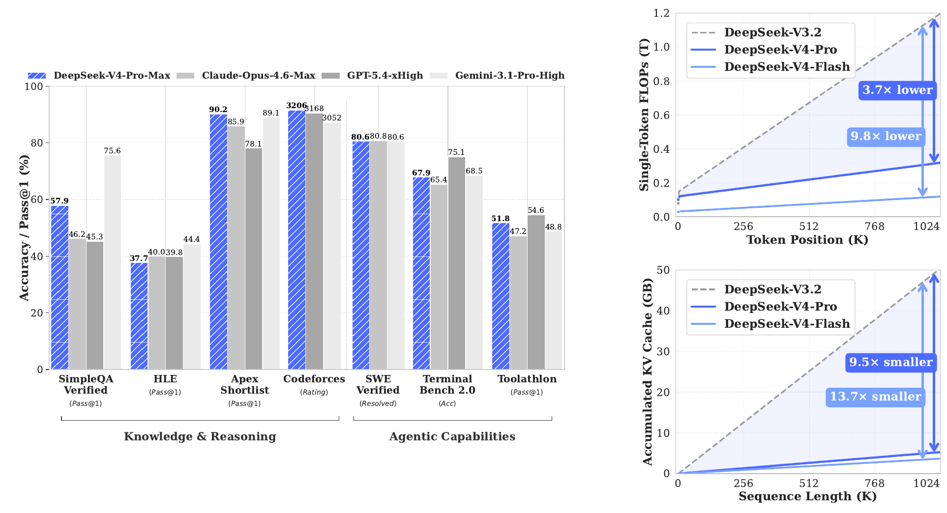
Start with the two plots on the right; they show what the whole report is aiming for.
The upper-right plot shows the compute needed to generate one token, with the token's position in the context on the horizontal axis. The previous generation, DeepSeek-V3.2, has a dashed line that climbs almost straight up: the later the position, the more expensive each token. At one million tokens, V4-Pro needs only 27% of V3.2's compute, and V4-Flash only 10%.
The lower-right plot is the KV cache. Again at one million tokens, V4-Pro needs only 10% of V3.2's, and V4-Flash only 7%.
It should be stressed that V3.2 already uses sparse attention, so it is not a wasteful baseline to begin with, and V4-Pro actually activates more parameters per token than V3.2. The gaps in these two plots therefore come mainly from the redesign of attention.
On the left, the strongest setting, DeepSeek-V4-Pro-Max, is compared with three closed models; we will come back to it in the discussion.
Solving the problem
Overall architecture
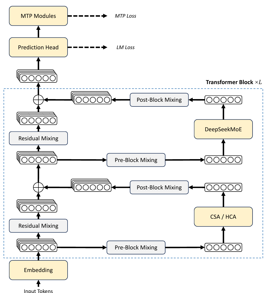
Most of it carries over from DeepSeek-V3. The feedforward layers are DeepSeekMoE, with shared experts and fine-grained routed experts; load balancing uses bias adjustment without an auxiliary loss; and multi-token prediction (MTP) is kept. There are two small changes. The function that computes routing affinity switches from Sigmoid to . And the first few layers, which used to be dense feedforward layers, are now MoE too, but with hash routing, which decides directly from the token ID which expert a token goes to.
The most eye-catching thing in the figure is that the residual stream is drawn as four stacked vectors. That is mHC.
mHC: widen the residual stream, then constrain it
A standard residual connection is . There is only one residual stream, and its width equals the hidden dimension .
Hyper-Connections (HC) widen the residual stream into copies, so the state becomes , and three small matrices decide how it is read and written:
mixes the residual copies into one, which becomes the layer's input; distributes the layer's output back to the residual copies; lets the residual copies mix with one another. The layer's own input and output are still -dimensional, so its internal design does not need to change, and since is far smaller than , the extra computation is small.
HC's problem is that numerics easily become unstable once many layers are stacked. The reason is not hard to see. Every layer multiplies by a , and if its spectral norm exceeds 1, the signal explodes after a few dozen layers of multiplication.
mHC (Manifold-Constrained HC) constrains to be a doubly stochastic matrix: all entries are nonnegative, and every row and every column sums to 1. The spectral norm of a doubly stochastic matrix is exactly 1, so it does not amplify the signal; the product of two doubly stochastic matrices is still doubly stochastic, so this holds no matter how many layers are stacked. and are constrained with Sigmoid to be nonnegative and bounded, preventing signals from canceling one another out.
Projecting an arbitrary matrix onto a doubly stochastic matrix uses the Sinkhorn-Knopp algorithm: first exponentiate so that every entry is positive, then alternately normalize the columns and the rows. V4 iterates 20 times. Let's try it with :
import numpy as np

rng = np.random.default_rng(0)
B_raw = rng.normal(scale=2.0, size=(4, 4))          # unconstrained residual mixing matrix (n_hc = 4)
print("Spectral norm before the constraint:", round(np.linalg.norm(B_raw, 2), 3))

M = np.exp(B_raw)                                     # exponentiate first so every entry is positive
for _ in range(20):                                   # t_max = 20
    M = M / M.sum(axis=0, keepdims=True)              # each column sums to 1
    M = M / M.sum(axis=1, keepdims=True)              # each row sums to 1

print("Row sums:", np.round(M.sum(axis=1), 4))
print("Column sums:", np.round(M.sum(axis=0), 4))
print("Spectral norm after the constraint:", round(np.linalg.norm(M, 2), 4))

x = rng.normal(size=4)
y = x.copy()
for _ in range(60):                                   # apply the same residual mixing 60 times, one per layer
    y = M @ y
print("Input norm:", round(np.linalg.norm(x), 3), " after 60 layers:", round(np.linalg.norm(y), 3))
Spectral norm before the constraint: 6.07
Row sums: [1. 1. 1. 1.]
Column sums: [1. 1. 1. 1.]
Spectral norm after the constraint: 1.0
Input norm: 1.286  after 60 layers: 0.297
Before the constraint, the matrix's spectral norm is 6.07, and multiplying it through 60 layers would give an astronomical number; after the projection it is 1.0, and after 60 layers the signal can only contract, never explode. To make the effect stand out, this example uses the same matrix for all 60 layers. In a real model, each layer's is different, but every one of them is doubly stochastic, so the conclusion is the same.
The actual , , and are generated dynamically from the input. is flattened and passed through RMSNorm and then a small linear layer; a static bias is added, the result is multiplied by a gating coefficient that starts out very small, and only then are the constraints above applied. Both V4 models use .
CSA and HCA: two kinds of compressed attention
Attention is the bottleneck for long context. V4 introduces two kinds of attention and interleaves them.
CSA (Compressed Sparse Attention) compresses first, then selects sparsely.
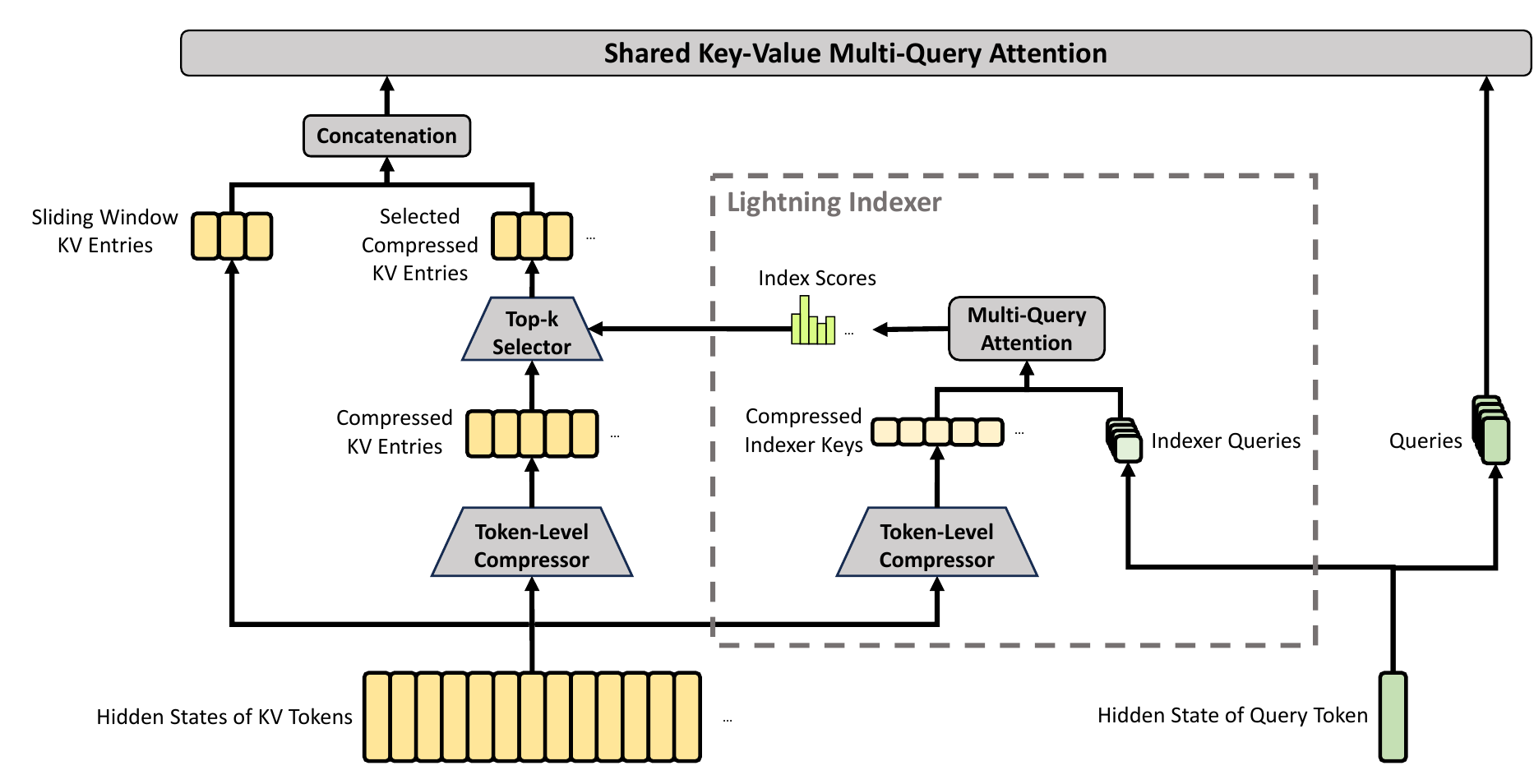
Read it from the bottom up.
The first step is compression. The KV of every tokens is compressed into one entry. The compression weights come from a learnable projection plus a positional bias passed through softmax, which amounts to a weighted average of those tokens. V4 sets .
The second step is selection. This carries over DeepSeek Sparse Attention (DSA) from V3.2: a lightweight lightning indexer scores every compressed entry and picks only the top . V4-Pro uses , and V4-Flash uses 512. The indexer itself runs in FP4 precision.
The third step adds back what is nearby. A compressed entry can only cover "whole earlier blocks" and cannot see the other tokens in its own block, and language models usually need the most recent context the most. So a separate sliding-window branch keeps the latest 128 uncompressed KV entries.
Finally, each KV entry serves as both key and value and is shared by all query heads, in the form of multi-query attention (MQA).
HCA (Heavily Compressed Attention) compresses much harder, squeezing every tokens into one entry, but does no sparse selection and looks at every compressed entry; it also adds a 128-token sliding window.
Let's count, for one million tokens, how many KV entries each query looks at:
| Attention | KV entries after compression | Entries each query actually attends to |
|---|---|---|
| Standard attention | 1,000,000 | 1,000,000 |
| CSA (, for Pro) | 250,000 | |
| HCA () | about 7,813 | about |
CSA relies on sparse selection: each query looks at only a little over a thousand entries, but picks them carefully out of 250,000 compressed entries. HCA does no picking, but each entry stands for 128 tokens, so it sees a rough outline of the whole context. Interleaved, the two split the work, one doing precise lookup and the other giving a global overview.
The size of the KV cache depends on how many entries have to be stored after compression. The report says that, against a common baseline of BF16 with 8-group GQA and a head dimension of 128, V4's KV cache at one million tokens is only about 2% of the baseline's. That figure also reflects other savings, such as storing the RoPE dimensions of KV entries in BF16 and the other dimensions in FP8, which saves almost half.
The report also lists several details that make this design trainable. Queries and KV entries each go through RMSNorm before attention, keeping attention logits from exploding; RoPE is applied only to the last 64 dimensions; and attention gets a learnable sink logit, letting a head's attention sum to less than 1.
The Muon optimizer
V4 switches most parameters to the Muon optimizer, while the embedding layer, prediction head, RMSNorm weights, and mHC's static biases still use AdamW.
The core of Muon is to "orthogonalize" the momentum matrix so that all singular values of the update are close to 1. Doing this exactly requires a singular value decomposition, which is too expensive, so it is approximated with Newton-Schulz iterations:
V4 uses a "hybrid" scheme of 10 iterations. The first 8 use , quickly pushing the singular values to near 1; the last 2 switch to , settling the singular values at 1.
Because the attention architecture already applies RMSNorm to queries and KV, attention logits do not explode, so V4 also has no need for QK-Clip, which other Muon implementations use to keep logits in check.
Pretraining
Configuration
| V4-Flash | V4-Pro | |
|---|---|---|
| Layers / hidden dimension | 43 / 4,096 | 61 / 7,168 |
| Routed experts (active per token) | 256 (6) | 384 (6) |
| CSA selection count | 512 | 1,024 |
| Total / active parameters | 284B / 13B | 1.6T / 49B |
| Training tokens | 32T | 33T |
Both use a CSA compression rate of 4 and an HCA rate of 128, with hash routing in the first 3 MoE layers. V4-Flash's first two layers use only sliding-window attention, while V4-Pro's first two layers use HCA; after that, CSA and HCA alternate.
Training starts at a sequence length of 4K and is gradually extended to 16K, 64K, and 1M. Sparse attention is not used from the start. V4-Flash warms up with dense attention for its first 1T tokens (V4-Pro's dense phase is longer), and sparse attention is added only at the 64K length, after a brief warmup of the lightning indexer. The learning rate stays constant most of the time and finally decays with a cosine schedule to one tenth.
In the post-training stage, the routed experts' weights and the indexer's QK path also go through FP4 quantization-aware training, saving further memory and compute.
Dealing with loss spikes
When training a trillion-parameter MoE, loss spikes are hard to avoid. The authors found that spikes are always tied to outliers in the MoE layers, and that the routing mechanism itself seems to amplify outliers, forming a vicious cycle. Simply rolling back only fixes things temporarily; the spikes come back.
They found two measures that work, and admit frankly that they don't yet understand why:
- Anticipatory Routing: at step , features are computed with the current parameters , but routing decisions are computed with somewhat older parameters , breaking the vicious cycle caused by the backbone and the router updating in sync. This adds about 20% to training time, so it is normally off. When the system detects a spike, it automatically rolls back briefly and turns this mode on for a while, then turns it off again.
- SwiGLU clamping: the linear branch of SwiGLU is clamped to , and the gate branch is capped at 10, suppressing outliers directly.
The authors say both measures worked in training both V4-Flash and V4-Pro, without affecting performance.
Comparing the base models
The authors compare three base models: V3.2, V4-Flash, and V4-Pro. V4-Flash is the most interesting. It has fewer active parameters and fewer total parameters than V3.2, yet beats V3.2 on most benchmarks, especially on knowledge and long-context tasks.
Post-training: from weight merging to distillation
Train a group of experts first
The first step of post-training resembles V3.2's. For each domain, run SFT and then reinforcement learning with GRPO, producing a group of expert models.
Reasoning effort is handled with experts too. V4 has three reasoning modes: non-thinking, Think High, and Think Max. Each mode is trained with a different length penalty and context length, and Think Max also injects an instruction at the start of the system prompt telling the model to "make maximum effort, no shortcuts," so that it writes out its entire reasoning.
For tasks that are hard to verify, V4 no longer trains a reward model that outputs a score. It uses rubrics together with a generative reward model (GRM) instead, and the policy model itself doubles as the GRM, so its ability to judge and its ability to generate are optimized together by reinforcement learning.
Distillation in place of merging
The next step is exactly what this note wants to highlight.
With a dozen or so experts in hand, how do you integrate their capabilities into a single model? Command A uses linear weight merging, and V3.2 uses mixed reinforcement learning. V4 uses neither, switching to multi-teacher on-policy distillation (OPD):
is the student being trained, is the -th expert, and is that expert's weight. "On-policy" means the training data is generated by the student itself, and each expert then gives its own probability distribution for every token the student wrote. The KL is the reverse one, , so on math problems the student naturally leans toward the math expert, and on coding problems toward the code expert.
The authors state their reason plainly: aligning knowledge at the logit level in practice avoids the performance degradation common in traditional weight merging or mixed reinforcement learning. This stage used a dozen or so teacher models to distill a single student.
On the details, common OPD implementations simplify the full-vocabulary KL to looking only at the sampled token at each position, using it as the advantage in reinforcement learning. This saves a lot of resources, but the gradient variance is high and training is unstable. V4 insists on full-vocabulary logit distillation, and for that it also has to solve the scheduling problem of a dozen or so teachers all providing full logits.
From Model Soups to Command A, the case for model merging has always been that it is cheap: no data, no training, just average. V4's choice shows that when you have the data and the compute, and the experts to integrate number a dozen or more with widely differing capabilities, paying for one distillation run to avoid merging's losses is worth it, at least for DeepSeek.
Context management during reasoning
A one-million-token context also changes how reasoning content is kept. V3.2 kept thinking content between tool calls, but discarded all earlier thinking as soon as the user sent a new message. In scenarios with tool calls, V4 keeps all the thinking content of the whole conversation, even across user messages; ordinary chat keeps the old approach. The tool-call format has also changed to an XML style, which the authors say reduces escape-character errors and tool-call failures.
Discussion
Results
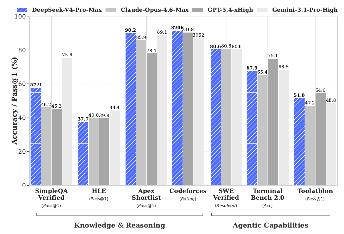
The hatched bars are V4-Pro-Max; the other three are the strongest reasoning settings of closed models.
On knowledge, V4-Pro-Max scores 57.9 on SimpleQA Verified, above Claude-Opus-4.6-Max's 46.2 and GPT-5.4-xHigh's 45.3, but clearly below Gemini-3.1-Pro-High's 75.6. On HLE it scores 37.7, slightly below the other three (40.0, 39.8, 44.4). On agent tasks, its 80.6 on SWE Verified is almost the same as the other models; on Terminal Bench 2.0 it scores 67.9, behind GPT-5.4-xHigh's 75.1.
This matches the authors' own summary: the best results among open models, with reasoning close to the frontier closed models, and agent tasks on par with the top open models but slightly behind the frontier closed models.
V4-Flash-Max does worse on knowledge because it has fewer parameters, but given a larger thinking budget, it can match V4-Pro on reasoning tasks.
Limitations in the authors' own words
The conclusion contains a very candid passage. To push long-context efficiency to the limit, V4's architecture is quite bold; to lower the risk, it also kept many previously validated components and small tricks, and the whole architecture ended up rather complex. The authors say the next step is more comprehensive and principled research to pare the architecture down to its most essential design. Anticipatory Routing and SwiGLU clamping work, but why they work is still unclear.
In addition, the report's title marks it as a "preview," most comparisons were run in the authors' own evaluation framework, and some of the agent-task comparisons come from internal evaluations.
Conclusion
DeepSeek-V4 uses two kinds of compressed attention to make a one-million-token context affordable: CSA compresses 4× and then carefully picks a little over a thousand entries, while HCA compresses 128× to see the global outline. mHC widens the residual stream and locks in stability with doubly stochastic matrices, and Muon speeds up convergence. As a result, at one million tokens, V4-Pro's per-token compute is only about a quarter of the previous generation's, and its KV cache only a tenth.
For the model-merging line of work, this report offers an interesting counterexample. Faced with the same job of integrating a group of experts into one model, Command A chose to average weights, while DeepSeek chose to let the student write for itself and have the teachers coach it token by token.
Merging's strength is that it is cheap; distillation's is that it is precise. DeepSeek clearly has the compute to afford the latter.