Original paper
Adafactor: Adaptive Learning Rates with Sublinear Memory Cost
- Publication
- ICML 2018Conference
- First submitted to arXiv
- arXiv:1804.04235
Cite this paper · BibTeX
The citation identifies the linked source version. It cites the original paper and its authors.
@misc{optimizersadafactor2018,
  title = {{Adafactor: Adaptive Learning Rates with Sublinear Memory Cost}},
  author = {Noam Shazeer and Mitchell Stern},
  year = {2018},
  eprint = {1804.04235},
  archivePrefix = {arXiv},
  url = {https://arxiv.org/abs/1804.04235}
}
Open the T5 paper to its training setup, and the optimizer line reads "For optimization, we use AdaFactor." It was later used for fine-tuning FLAN and Flan-T5, too, and for pre-training the 540-billion-parameter PaLM.
Go back to the source, and the Adafactor paper has just one experimental task, an English-to-German Transformer, with each training run taking under two hours on a single TPU v2. The problem Noam Shazeer and Mitchell Stern set out to solve is stated on the first page. Adam uses too much memory.
Defining the problem
Adam stores two extra numbers for every parameter, the first moment and the second moment . The paper says this triples the memory requirement, with one copy each for the weights, and . Take a feed-forward weight matrix. It has 4,194,304 parameters, so Adam has to store another 8,388,608 numbers.
In 2018, the authors observed that compute was growing much faster than memory capacity, and memory had become one of the limits on model size. Counting only weights and optimizer state, Adam's two extra copies mean the same memory can hold a model only a third as large.
The authors set out to do four things:
- shrink the second moment from numbers to ;
- drop the first moment, ;
- deal with the instability that shows up once momentum is gone;
- make the step size proportional to the scale of the parameters.
The first two save memory, the third is the trouble those savings create, and the fourth is an improvement the authors threw in along the way.
Solving the problem
Keep only row sums and column sums
Suppose a layer's weights form an matrix. Adam maintains an exponential average of the squared gradients, , of the same size. If we store only two small matrices and with , the memory shrinks a lot. The question is how to factor it.
The most common low-rank approximation is truncated SVD, which is optimal under the Frobenius norm, but it has two problems. First, the top singular vectors don't decompose over addition. The singular vectors of a sum of two matrices bear no simple relation to those of each matrix, so it can't be combined with an exponential average. Second, the approximated entries can be negative, while Adam needs to take the square root of and then its reciprocal.
The authors turn instead to the generalized KL divergence common in nonnegative matrix factorization, also called I-divergence:
It is never less than 0, and equals 0 only when . The goal is to minimize subject to and both being nonnegative. General rank requires alternating optimization; rank 1 has a closed-form solution (Lemma 1 in the paper):
is the sum of each row, is the sum of each column, and the denominator is the sum of all entries. In plain terms, the estimate at row , column is "sum of row × sum of column ÷ total sum."
Let's work through a example:
The top-left entry is and the bottom-right is , so the whole matrix comes back intact, because the second row happens to be a third of the first, which makes itself rank 1. Change the bottom-right 2 to 8, and the row sums become , the column sums and the total 30, so the bottom-right estimate is only . The factorization remembers the overall size of each row and each column, but not that one particular cell stands out.
This solution uses only the row sums and column sums, both linear functions of , so "average, then sum" equals "sum, then average." In practice, you just keep exponential averages of the row sums and column sums directly, without ever reconstructing the full . For that weight matrix, the second moment goes from 4,194,304 numbers to 5,120.
The authors write the version as Algorithm 2:
and then update with , as in Adam. Biases and other vector-shaped parameters keep the original element-wise , since they're small to begin with.
Drop the momentum, and things break
The second step is simpler. Set , and don't store at all.
All the experiments use a Transformer on WMT'14 English-to-German, for 100,000 steps, with each batch holding about 4,096 source tokens plus 4,096 target tokens, roughly an eighth of the original Transformer paper's batch. Each setting is run twice, once with warmup, at learning rate , and once without, starting directly at . The metric is BLEU on the newstest2013 dev set.
| Setting | With warmup | No warmup |
|---|---|---|
| (A) Adam, | 25.6 | 0.1 |
| (B) Adam, | 25.4 | 23.1 |
| (C) Factored second moment, | 25.4 | 0.2 |
| (D) Row means only | 25.2 | 0.3 |
| (E) Column means only | 0.3 | 0.5 |
Compiled from Table 2 of the paper; all settings use .
With warmup, dropping momentum (A versus B) and then factoring the second moment (C) change BLEU by only a few tenths. (D) and (E) are two even leaner controls that store only the row means or only the column means. Row means do about as well as the baseline, while column means break down entirely. The authors' explanation is that this model's word embeddings and output softmax share one weight matrix, with each row corresponding to a token; rows for frequent tokens get far larger gradients than rows for rare ones, and storing only column means lumps every token onto the same scale.
The trouble is in the right-hand column. Without warmup, (B), with momentum, still gets 23.1, while (A), without momentum, drops straight to 0.1.
Stale second moments
The authors suspect . A small means the second moment decays fast, which Reddi et al. had already shown causes convergence problems; a large means the estimate comes from gradients long past, and it can't keep up when the model changes quickly.
Both show up. At it's 25.6 with warmup and 0.1 without; at the two are 18.4 and 15.6, stable but not learning well.
To check whether the estimate is lagging, the authors define a quantity:
is the update before it's multiplied by the learning rate. If is estimated accurately, each parameter's should be around 1, and the RMS over the whole matrix should be close to 1 as well.
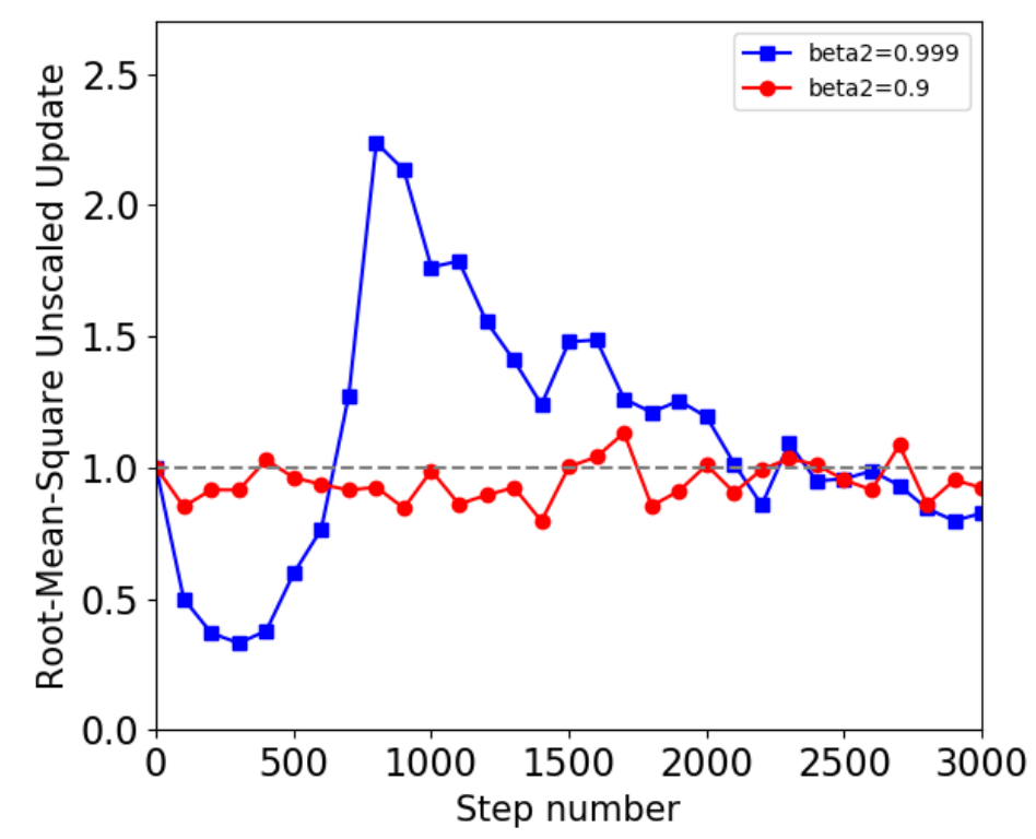
The red line is , staying around 1 throughout. The blue line is . It first drops to about 0.33 over the first 300 steps, meaning updates smaller than expected; then around step 800 it spikes to 2.24, with updates more than twice as large as expected. Both runs had warmup and neither diverged, so this isn't a case of training blowing up and then producing larger updates; the authors think the oversized updates cause the instability, and admit that this figure is only supporting evidence, not proof.
Update clipping
If the problem is updates that are too large, then limit the update directly:
When the RMS exceeds the threshold , the whole matrix's update is scaled down proportionally to . This differs from the usual gradient clipping. Gradient clipping limits the gradient, but methods like Adam then divide each parameter by , so once goes stale, a clipped gradient can still be blown up into a huge update; update clipping limits the step that actually gets applied.
With , the no-warmup 0.1 is rescued to 21.5; at the threshold is too loose, and it's still only 0.2. With warmup, clipping makes no clear difference either way.
Let rise with the step count
Another route is to make small at first and large later. The authors first point out that Adam's bias correction is itself equivalent to an increasing :
It is 0 at , then gradually approaches . The authors propose a different schedule:
With the the paper adopts, it's 0.84 at step 10, 0.975 at step 100 and 0.996 at step 1,000, passes 0.999 around step 5,600, and is 0.9994 at step 10,000. Early in training it behaves like fast decay, which is stable; later it behaves like slow decay, which gives more accurate estimates.
This schedule has two more benefits. , so the weights on all past gradients sum to exactly 1, and no bias correction is needed. Also, using the convergence condition for infinite products, the authors show that only lets the weight on every old gradient eventually go to 0; with , rises too fast, and early gradients keep a sizable share forever. is exactly the arithmetic mean of all squared gradients.
| Setting | With warmup | No warmup |
|---|---|---|
| (G) | 18.4 | 15.6 |
| (H) , clipping | 25.4 | 21.5 |
| (I) , clipping | 25.7 | 0.2 |
| (J) Factored, , clipping | 25.6 | 22.4 |
| (K) | 25.6 | 21.1 |
| (L) | 25.6 | 0.1 |
| (N) , clipping | 25.9 | 22.4 |
Compiled from Table 2 of the paper; all with .
on its own holds up without warmup; on its own isn't enough and needs clipping too. (N) gets the table's highest with-warmup score, 25.9, and (J) shows that a factored second moment plus clipping can be about as stable as Adam with momentum.
Relative step size
The last piece has nothing to do with memory. Adam's learning rate is an absolute step size; the authors think the relative change in the parameters matters more, so they multiply the step size by the parameters' own scale:
is the current root mean square of this parameter matrix, and is a floor, so that parameters initialized to 0 can still leave the origin. The paper's acknowledgments specifically credit Geoffrey Hinton's view that training goes smoothly when each update is about to times the size of the parameters.
The authors tested three word-embedding initializations (50,000 steps, batches of 16,384 tokens, embeddings not shared with the softmax). The original Transformer initializes with standard deviation and multiplies by at compute time, so the same absolute learning rate suits both the embeddings and the other weights; Adam gets 26.4 and Adafactor 26.6. With the more naive initializations, Adam drops to 25.8 and 24.2, while Adafactor still gets 26.4 and 25.4. When the parameter scale is poorly set, relative step sizes suffer less.
Putting it together
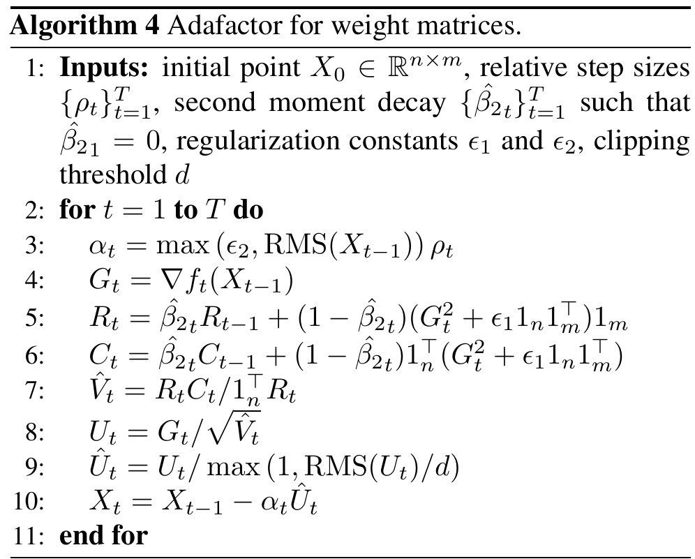
Chain the five pieces together and you get Algorithm 4. Line 3 is the relative step size, lines 5 and 6 are the row-sum and column-sum averages with added, line 7 reconstructs the second moment, and line 9 is update clipping. The paper's recommended hyperparameters are , , , and , with no momentum. For an matrix, the whole optimizer stores only extra numbers.
Discussion
The full version's scores
| Setting | With warmup | No warmup |
|---|---|---|
| (A) Adam, | 25.6 | 0.1 |
| (B) Adam, | 25.4 | 23.1 |
| (O) Adafactor | 25.0 | 25.5 |
| (P) Adafactor with momentum added back | 24.9 | 25.3 |
| (Q) SGD, best learning rate | 24.3 | 9.1 |
Compiled from Table 2 of the paper; (O) and (P) use the relative step size , and (Q) uses with warmup and without; every larger learning rate diverged without warmup.
The full Adafactor gets the table's highest no-warmup score, 25.5, and 25.0 with warmup, 0.6 below (A) without momentum and 0.4 below (B) with momentum. The authors themselves note that the relative step sizes can't be compared directly with the step sizes in the other rows, so they can't tell whether the stability comes from the relative step size. SGD also uses no extra memory, but its best is only 24.3, and it's very sensitive to the learning rate.
These results come from just one translation task, one model, 100,000 steps, and a batch eight times smaller than the original setup. The paper ends by saying the saved memory "should enable training of significantly larger models," but it has no large-model experiments at all, and no measurements of memory or speed.
Adafactor after the paper
The real large-scale tests were done by others.
T5 adopted Adafactor directly. Its pre-training learning rate is held at 0.01 for the first ten thousand steps and then decays as the inverse square root, which is exactly this paper's . T5's published training config also keeps the paper's , an update clipping threshold of 1.0, the factored second moment and parameter scaling.
DeepMind tried another direction while training Gopher. At 1.4 billion parameters, Adafactor was stable and worked well, but at 7.1 billion it began to show mild loss divergence; Adam's maximum learning rate was , and Adafactor was still unstable even at . They still ended up fine-tuning Gopher with Adafactor, because its hardware requirements are much lower.
When Google trained the 2-billion-parameter ViT-G, they said Adafactor "did not work out of the box" and changed three things. They added back a half-precision first moment, disabled step-size scaling relative to the weight norm, and capped at 0.999. After the changes, it performed on par with or slightly better than Adam.
PaLM was more direct. The paper states that it uses Adafactor "without factorization," which is effectively Adam with parameter scaling; momentum is , the second moment uses , and the learning rate is for the first ten thousand steps, then decays as . They specifically explain that this schedule is more stable than a fixed 0.99, because embeddings of rare tokens can have poorly estimated second moments over short windows.
Update clipping also got carried off on its own. In 2023, Wortsman et al. found that loss spikes in large CLIP training always came 1 to 8 steps after the second moment underestimated the squared gradient, and proposed StableAdamW, which "is AdamW with the update clipping technique introduced in AdaFactor." They also wrote that large-scale training has largely moved away from Adafactor in its original form, speculating that the reason is the factored second moment or the lack of momentum.
On the library side, Hugging Face Transformers has had Adafactor for a long time, while PyTorch only added torch.optim.Adafactor in version 2.5. Both use relative step sizes by default (Hugging Face lets you turn this off); PyTorch's version treats lr as the upper bound on , and notes that it deliberately departs from the paper in where goes.
Conclusion
Adafactor uses a rank-1 factorization by row and column sums to shrink the second moment from to , then drops momentum. The authors traced the resulting instability to stale second moments, and handled it with update clipping and a schedule for . All this held on one translation task, and later held up at T5's scale too; at billions of parameters, Gopher reported it unstable, and PaLM and ViT-G put momentum back.
If you use Adafactor in Hugging Face and want to control the learning rate yourself, remember to set relative_step=False and scale_parameter=False. Otherwise the optimizer will switch to its built-in , or multiply your learning rate by the parameters' RMS, and the learning-rate schedule you wrote won't take effect as written.
The Adafactor that PaLM used ended up dropping even the factor.