Original paper
WSM: Decay-Free Learning Rate Schedule via Checkpoint Merging for LLM Pre-training
- Publication
- ICLR 2026Conference
- First submitted to arXiv
- arXiv:2507.17634
Cite this paper · BibTeX
The citation identifies the linked source version. It cites the original paper and its authors.
@misc{modelmergingwsm2025,
  title = {{WSM: Decay-Free Learning Rate Schedule via Checkpoint Merging for LLM Pre-training}},
  author = {Changxin Tian and Jiapeng Wang and Qian Zhao and Kunlong Chen and Jia Liu and Ziqi Liu and Jiaxin Mao and Wayne Xin Zhao and Zhiqiang Zhang and Jun Zhou},
  year = {2025},
  eprint = {2507.17634},
  archivePrefix = {arXiv},
  url = {https://arxiv.org/abs/2507.17634}
}
When training large language models, the learning-rate schedule has always been a troublesome setting.
The traditional cosine schedule needs to know the total number of training steps from the very start just to draw its curve; if you want to train on more data, you have to start over. WSD (Warmup-Stable-Decay) inserts a stable phase with a constant learning rate in the middle, so you can branch off from the stable phase and anneal at any time. DeepSeek-V3 and ERNIE 4.5 both use it.
But WSD still leaves a pile of things to decide in advance: when to start annealing, how many tokens to anneal on, and which decay curve to use. If you want to keep training after annealing, you have to go back to the state before annealing and replan.
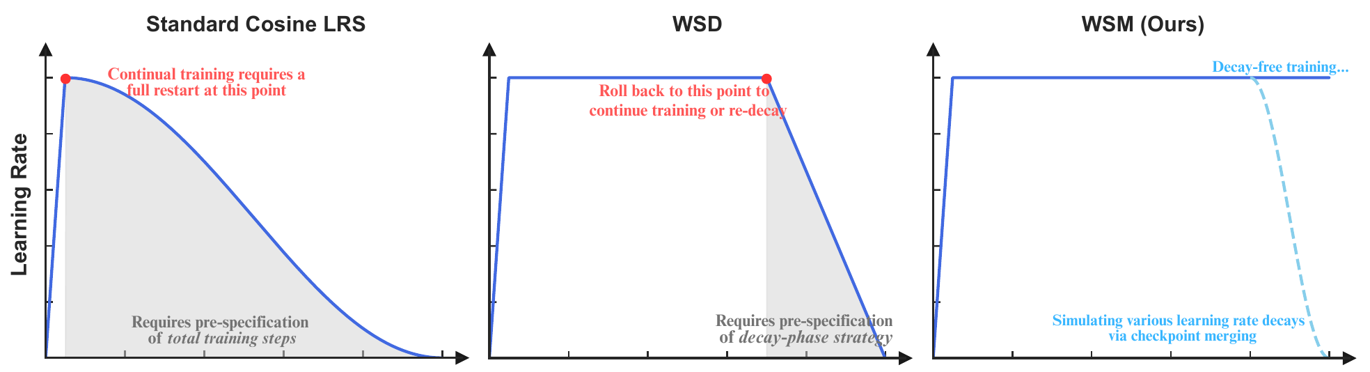
This paper, from Ant Group's Ling team and Renmin University of China, sets out to remove the decay phase entirely. After warmup, the learning rate stays constant, and the effect of annealing comes from merging checkpoints instead. They call this schedule WSM (Warmup-Stable and Merge).
Defining the problem
Around the same time, ByteDance Seed's PMA had already found that averaging checkpoints during the constant-learning-rate phase yields scores close to, or even matching, those of annealed models.
But the relationship between "averaging" and "annealing" had never been spelled out. How much weight should each checkpoint get when averaging? What kind of annealing do equal-weight averaging and an exponential moving average correspond to? If this relationship could be written down as a formula, merging could simulate any decay curve already known to work well.
Solving the problem
Writing merging as decay
Suppose there are checkpoints saved in order, . The merged model is
This expression shows no obvious connection to the learning rate. The authors rewrite it by expressing each checkpoint as "starting point plus the updates that follow." Let be the update at step (already multiplied by the learning rate), so that . Then
Substitute this back into the merging formula and swap the order of the two sums. The -th update appears in every checkpoint with , so
where .
The result is intuitive. Merging checkpoints is equivalent to starting from and adding back each subsequent update multiplied by a coefficient . Since is a tail sum of the , it necessarily decreases with , and that is exactly a decaying learning-rate curve.
It works in reverse too. For any desired decreasing decay curve , the corresponding checkpoint weights are uniquely determined as
This is Theorem 3.1 of the paper.
Running the numbers
Let's walk through both directions with a small example. First, see which decay equal-weight averaging of 5 checkpoints corresponds to; then go the other way and compute the weights a 1-sqrt decay needs; finally, confirm that both sides really give the same result.
import numpy as np

def merge_weights_from_decay(w):
    """Theorem 3.1: recover checkpoint weights c_0..c_k from gradient decay coefficients w_1..w_k."""
    k = len(w)
    c = np.zeros(k + 1)
    c[k] = w[-1]
    for j in range(1, k):
        c[j] = w[j - 1] - w[j]
    c[0] = 1 - w[0]
    return c

rng = np.random.default_rng(0)
k = 4
theta_n = rng.normal(size=3)
g = rng.normal(size=(k, 3)) * 0.1            # k updates at a constant learning rate
ckpts = [theta_n - g[:j].sum(0) for j in range(k + 1)]   # θ_n, θ_{n+1}, ..., θ_{n+k}

# 1) Which decay does averaging the latest 5 checkpoints correspond to?
c_mean = np.full(k + 1, 1 / (k + 1))
w_equiv = [c_mean[i:].sum() for i in range(1, k + 1)]
print("Average of 5 checkpoints → effective multiplier per update:", np.round(w_equiv, 2))

# 2) For a 1-sqrt decay, what checkpoint weights do we need?
t = np.arange(1, k + 1) / (k + 1)
w_sqrt = 1 - np.sqrt(t)
c_sqrt = merge_weights_from_decay(w_sqrt)
print("1-sqrt decay multipliers:", np.round(w_sqrt, 3))
print("Matching checkpoint weights:", np.round(c_sqrt, 3), " sum", round(c_sqrt.sum(), 6))

merged = sum(cj * th for cj, th in zip(c_sqrt, ckpts))
decayed = theta_n - (w_sqrt[:, None] * g).sum(0)
print("Max difference between merged and decayed results:", np.abs(merged - decayed).max())
Average of 5 checkpoints → effective multiplier per update: [0.8 0.6 0.4 0.2]
1-sqrt decay multipliers: [0.553 0.368 0.225 0.106]
Matching checkpoint weights: [0.447 0.185 0.142 0.12  0.106]  sum 1.0
Max difference between merged and decayed results: 1.3877787807814457e-17
The first line shows that equal-weight averaging of 5 checkpoints is equivalent to multiplying the 4 subsequent updates by 0.8, 0.6, 0.4, and 0.2 respectively, which is a linear decay. The third line is the result of going in reverse. To simulate a 1-sqrt decay, the oldest checkpoint gets the largest weight, 0.447, and the rest decrease in turn. The difference in the last line is within floating-point error, so both computations arrive at the same parameters.
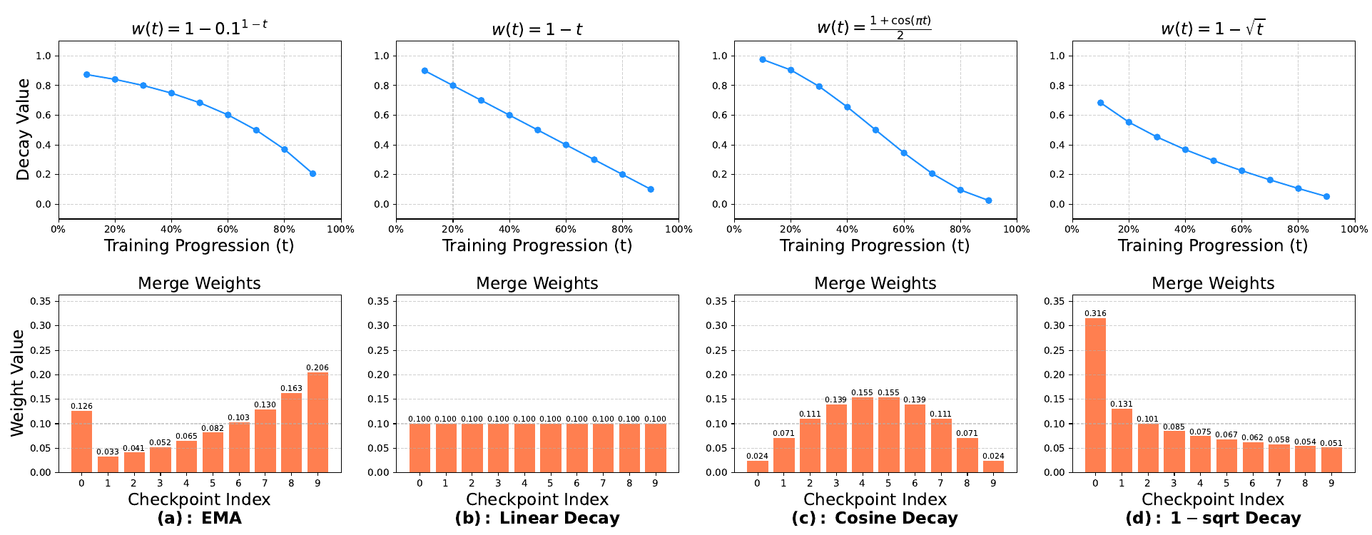
The paper converts four common merging schemes into decay curves. The most interesting is EMA. EMA gives newer checkpoints more weight, which seems perfectly reasonable, yet it works out to a convex decay curve that barely drops at first and only plunges at the very end.
The WSM pipeline
With this correspondence in hand, the WSM pipeline has three steps.
- Warm up to the peak learning rate, then keep it there.
- At some point in training, you can switch the data to curated high-quality data, matching the usual practice of "annealing data."
- Save a checkpoint every fixed number of tokens. A separate asynchronous process keeps taking the latest checkpoints, computes weights according to the decay curve to be simulated, and merges them.
Training itself never stops, and a merged model is available for evaluation or delivery at any time.
The authors also compared offline and online merging. Offline merging, which keeps every checkpoint, lets you try different decay curves and window sizes after the fact; once the best setting is found, you can switch to an online version that keeps only the latest checkpoints. The main cost is storage space, and in the authors' experiments was already enough.
Discussion
Experimental setup
The model is Ling-mini, an MoE with 16.3B total parameters and 1.4B active parameters. The architecture is 1 dense layer plus 19 MoE layers, each choosing 8 of 256 experts, plus 1 shared expert. The optimizer is AdamW, with a peak learning rate of 4.78e-4 and a batch size of 2048.
The starting point is a checkpoint trained at a constant learning rate on 10.2T tokens, 10T of it standard-length data and 200B long-context data. From there, training switches to high-quality annealing data and splits into two branches, each trained on 400B tokens:
- WSD: decay the learning rate as usual.
- WSM: keep the learning rate constant, save a checkpoint every 25B tokens, and merge the latest several with equal-weight averaging.
Better than WSD
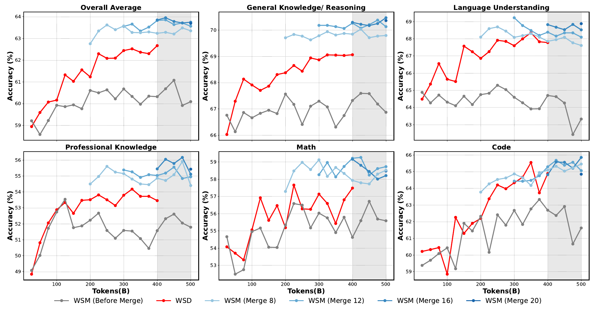
Look at the gray and blue lines first. The gray lines are unmerged checkpoints at a constant learning rate, and their scores stay stuck low; after merging, the blue lines jump right above the red line. In the overall-average plot, red WSD reaches about 62.7 at 400B, while the blue lines mostly sit between 63 and 64.
The gray region beyond 400B is another advantage of WSM. WSD's decay ends at 400B, and training any further means replanning; WSM's learning rate never came down, so training can simply carry on.
When the best checkpoint from each side is compared, WSM is 1.3 points higher on average. Math, code, and professional knowledge all improve; on individual benchmarks, MATH gains 2.7 points, HumanEval 2.4, and MMLU-Pro 2.1.
The advantage holds up after SFT. With both base models given 5 epochs of SFT under identical settings, WSM's overall average is 64.07 and WSD's is 62.90; code is the exception, where WSM actually comes out 0.28 points lower.
Predicting annealing at any point in time
Throughout pretraining, the authors also ran a comparison at 2T, 4T, 6T, 8T, and 10T tokens. One side runs a real 100B-token anneal; the other averages 4 checkpoints taken within the preceding 100B tokens.
This time general pretraining data is used rather than high-quality annealing data, so WSM's advantage is less pronounced, but the two scores track each other closely all the way. WSM can therefore also serve as an estimate of "how good it will be after annealing," without opening an annealing branch every time.
Which factor matters most
Merging method. Weights that simulate 1-sqrt decay, equal-weight averaging, and EMA give overall averages of 64.06, 63.95, and 63.01 respectively, all above WSD's 62.67. 1-sqrt slightly beats equal-weight averaging, and EMA is clearly the worst.
This matches experience with annealing. In their WSD experiments, the authors also found that the concave 1-sqrt curve and the linear curve beat convex curves, and EMA corresponds precisely to a convex decay.
Merging duration. The more tokens the merging window covers, the better the performance, though the gains gradually shrink. This also mirrors annealing: past a certain point, adding more annealing data does little. EMA, on the other hand, shows no visible effect of window size at all.
Merging granularity. With the merging duration fixed at 80B tokens, the authors compare save intervals: saving every 5B and merging 16, every 10B and merging 8, every 20B and merging 4, and every 40B and merging 2 give overall averages of 63.63, 63.78, 63.36, and 62.77 respectively, while taking a single checkpoint gives 60.33. Finer granularity gets closer to a continuous decay curve, but the differences are far smaller than those caused by duration.
The authors therefore consider merging duration the most critical factor, with a larger effect than either the save interval or the number of checkpoints merged.
Merging plus decay adds nothing
Since merging can simulate decay, can the two be stacked? The authors tried decaying and then merging, as well as merging and then decaying, and neither brought any extra improvement. The model that merged and then decayed was better at first, but in the end the two came out even.
The authors' reading is that merging and decay are two roads to the same goal: interchangeable, but not additive.
A side effect on MoE
The last observation concerns MoE load balancing. WSM models show clearly smaller deviations in expert load: the maximum deviation drops from 0.601 to 0.545, and the minimum from 0.322 to 0.201. The language-model loss, however, is slightly higher, 0.697 against 0.675. Merging makes expert usage more even at the price of a slightly worse loss, and the paper does not go on to separate how each of these affects downstream scores.
Scope of the evidence
The main experiments use a single 16B MoE model, starting from a checkpoint already trained on 10.2T tokens. The WSD baseline uses the 1-sqrt decay, which performed best among the decays the authors compared in the appendix, making the comparison fairer; but there is only one annealing length, 400B tokens, and the paper does not say whether the gap would be as large at other lengths. The +3.5% MATH and +5.5% MMLU-Pro in the abstract are relative gains; in percentage points they are the 2.7 and 2.1 reported in the main text.
The Ling team's later Ling 2.0 technical report also adopts the WSM schedule.
Conclusion
WSM uses a derivation that swaps the order of summation to connect checkpoint merging with learning-rate decay. The tail sums of the merge weights are the decay coefficients, and conversely, merge weights can be computed from any decreasing decay curve.
In practice, the learning rate is no longer adjusted after warmup, and annealing is left to merging. Training can go on indefinitely, a "post-annealing" model is available at any point, and in the authors' experiments it even comes out a little better than WSD.
Don't reach for EMA just yet. It looks like the most convenient choice, yet it works out to the convex curve that performs worst.