Original paper
The Road Less Scheduled
- Publication
- NeurIPS 2024Conference
- First submitted to arXiv
- arXiv:2405.15682
Cite this paper · BibTeX
The citation identifies the linked source version. It cites the original paper and its authors.
@misc{optimizersschedulefree2024,
  title = {{The Road Less Scheduled}},
  author = {Aaron Defazio and Xingyu Alice Yang and Harsh Mehta and Konstantin Mishchenko and Ahmed Khaled and Ashok Cutkosky},
  year = {2024},
  eprint = {2405.15682},
  archivePrefix = {arXiv},
  url = {https://arxiv.org/abs/2405.15682}
}
On August 1, 2024, MLCommons announced the results of the first AlgoPerf training algorithms competition.
If you haven't heard of AlgoPerf, it pits optimizers and training procedures themselves against each other. The models, data and hardware (8 V100s) are all fixed, and the question is who can train 8 workloads to a specified validation score the fastest, with workloads spanning machine translation, image classification, MRI reconstruction, speech recognition, molecular graphs and click-through-rate prediction. There are two rulesets. In external tuning, you can supply a hyperparameter search space, and the organizers sample 5 configurations from it for you to try; in self-tuning, no hyperparameter search is allowed outside of training, so the method has to handle every workload by itself within a single run. The most common approach is a single configuration for everything. As compensation, the training-time limit is tripled.
In self-tuning, only one submission beat the organizers' baseline. That was Schedule Free AdamW, submitted by researchers from Meta and Samsung, with a score of 0.8542; the baseline, NAdamW with linear warmup and cosine decay, scored 0.8194, and the other four entries were all below 0.4. The method's defining feature is that it uses no learning-rate schedule at all, and doesn't need to know in advance how many steps it will train for.
The paper behind it is called The Road Less Scheduled, a title borrowed from the "less traveled" line in Frost's The Road Not Taken, and the conclusion section really does quote the poem. The first author is Aaron Defazio of Meta FAIR, whose earlier D-Adaptation also tackled the question of how to set the learning rate. The code went up on PyPI as the schedulefree package in April; the paper didn't reach arXiv until the end of May.
Defining the problem
Schedules need an endpoint
The most common learning-rate schedules today are cosine and linear decay, and both require knowing the total number of steps before the curve can be drawn. Getting wrong is costly. Chinchilla's appendix measured that setting the cosine cycle more than 25% longer than the actual number of steps makes the model noticeably worse; and if you want to extend training partway through, you have to replan.
Averaging: great in theory, poor in practice
The other route is to skip the schedule and average the parameters instead. Polyak–Ruppert averaging is the most classical approach. SGD runs as usual with a fixed step size, and a separate average of all the points visited is maintained:
makes exactly the equally weighted average of . By classical convergence theory, for convex Lipschitz problems you should return , not the last iterate . In practice, this average does much worse than SGD's last iterate, which the authors describe as folklore in the field of optimization.
Recent theory has further shown that a linear-decay schedule on its own lets the last iterate achieve the optimal worst-case rate. In theory, schedules and averaging play much the same role, but a schedule has to know up front. So the authors ask whether there exists an averaging method that matches schedules in practice without giving up the theoretical guarantees.
Solving the problem
Three sequences
The Schedule-Free SGD update is Eqs. (3) to (5):
Starting from , the three sequences divide up the work:
- is the base sequence, where the underlying optimizer takes its steps; here, that's plain SGD.
- is the evaluation sequence, the equally weighted average of , and also the model you hand over at the end.
- is where the gradient is computed, interpolating between and .
Compared with Polyak–Ruppert averaging, only the first line is new. The gradient is computed not at but at , between and .
The two extremes
controls which side leans toward. At , , the gradient is computed at , and this is Polyak–Ruppert averaging. At , , and the gradient is computed at the average; this is called primal averaging, and it too has optimal worst-case guarantees, but it is generally considered too slow to converge to be practical.
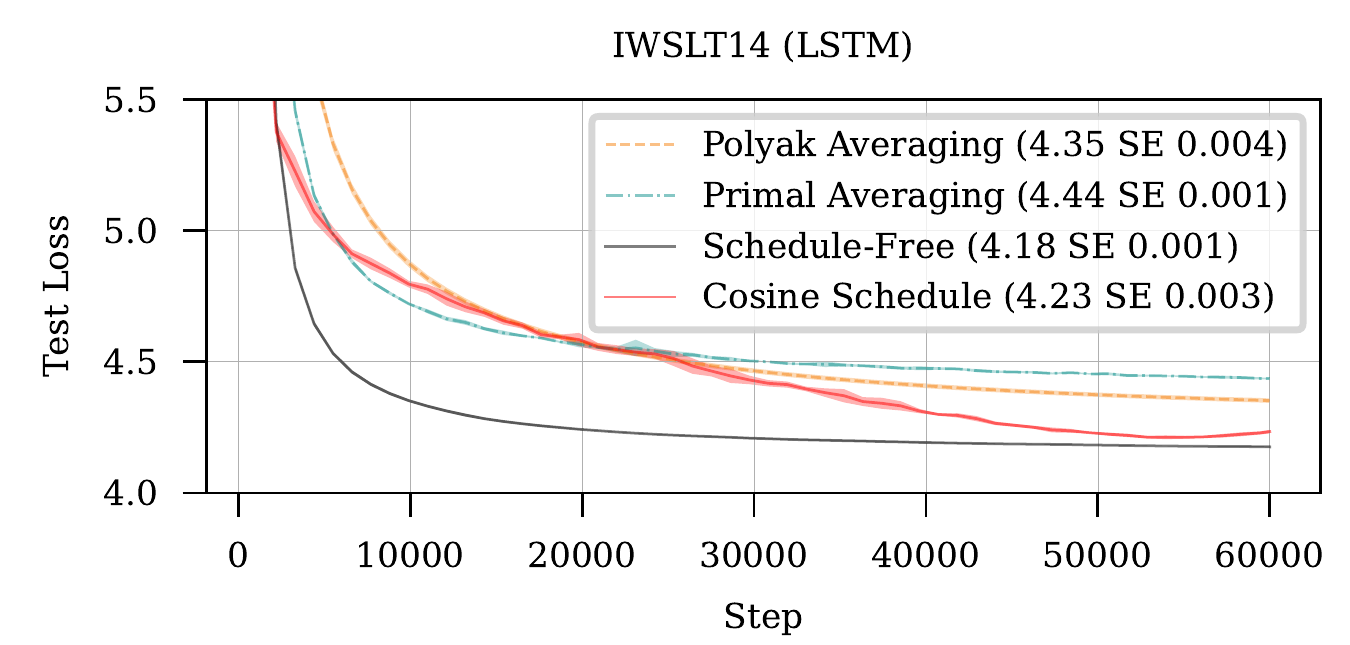
This plot is an LSTM on IWSLT14 German-to-English. Both extremes lose to a tuned cosine schedule, with Polyak averaging ending at 4.35, primal averaging at 4.44 and cosine at 4.23. Schedule-Free takes the middle ground with , ends at 4.18, and drops faster than anything else over the first 10,000 steps.
The authors' explanation is that moves faster than , so the interpolation keeps the fast convergence of Polyak averaging; meanwhile is pulled toward , which keeps the gradient location from straying too far from the model being returned and adds stability.
A different kind of momentum
plays a role much like momentum, and the paper compares it with ordinary exponential moving average (EMA) momentum. When the gradient from step enters , its immediate effect is , which is at , the same as EMA momentum. The difference lies in the remaining 90%. EMA momentum adds most of it within roughly the next 10 steps; Schedule-Free feeds it in very slowly through the average .
This kind of momentum has no theoretical downside. Theorem 1 says that if is convex, every per-sample loss is -Lipschitz, and samples are i.i.d., then taking (where is the distance from the starting point to the optimum), for any in :
This is the optimal rate for non-smooth convex problems, down to the constant. EMA momentum, by contrast, actually worsens the worst-case guarantee in the same setting.
Isn't just a decaying schedule?
By now you might be wondering whether the in the update for is just a decreasing learning rate in disguise.
In a sense, yes. The authors use Figure 4 to show how much of each step's gradient ends up in and in :
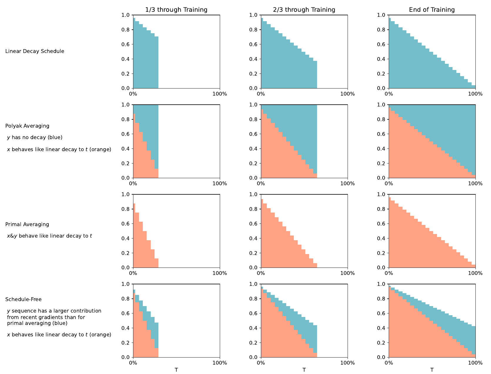
Start with the first row. At 1/3, 2/3 and the end of a linear-decay schedule, each step's gradient is added to the parameters according to the learning rate at the time, and later steps are smaller, so you get a ramp; but this ramp's endpoint is fixed at .
Now look at the orange parts of the three rows below, which are . For all three averaging methods, at every point in time looks like a linear decay that ends right at the current . That is why averaging can replace a schedule. It implicitly contains one, except that this schedule's endpoint moves forward with , so doesn't need to be known in advance.
The blue parts are , and this is where the three methods differ. For Polyak averaging, is just , every step's gradient counts in full, and late in training, recent gradients carry far more weight than under a schedule; for primal averaging, is just , recent gradients are squashed small, and early convergence is slow; Schedule-Free sits in between, giving recent gradients a modest boost.
Appendix B writes this out algebraically. Let be one step of the base optimizer, and . Then with equal-weight averaging and a fixed , the actual movement of at each step is:
That is, a momentum term plus times the base step. If is allowed to vary over time and is chosen to be exactly , the coefficient on the momentum term vanishes entirely, and what remains is a linear-decay schedule. Schedule-Free opts for a fixed , so it doesn't need .
How far the theory reaches
Theorem 1 is actually a special case of the more general Theorem 2. Theorem 2 allows any online learning algorithm to produce , with any averaging weights and interpolation coefficients , and turns their regret into a convergence guarantee for stochastic optimization, a form of online-to-batch conversion. Setting gives classical Polyak averaging, gives primal averaging (which Defazio's earlier work showed is equivalent to heavy-ball momentum), and gives the last-iterate guarantee of the linear-decay schedule. Appendix C then tightens it into an equality and derives accelerated rates for smooth problems.
The conditions should be spelled out too. These guarantees are all for convex problems; Theorem 1's step size still has hidden inside it, and switching to the anytime version works poorly in practice. What people actually use is a much larger fixed step size, . Theorem 3 shows that under a condition that can be checked during training, even this large step size achieves the optimal rate; the authors checked it on every problem in Section 4.1 and it held, but they also admit there's no complete understanding yet of when large step sizes work for stochastic problems.
Further support comes from quadratics. The authors randomly generated 10 quadratic problems in 20 dimensions and swept and . With small step sizes, makes almost no difference; with large ones, is the key to converging.
Schedule-Free AdamW
Swap the base optimizer for AdamW, and you get Algorithm 1:
- , interpolation in place of momentum.
- Compute the gradient at .
- .
- , folding both warmup and bias correction into the learning rate.
- .
- .
- .
It differs from AdamW in a few places.
- No first moment. goes to the interpolation instead, so only , and need to be stored, the same memory as AdamW; the SGD version likewise matches SGD with momentum.
- Warmup is still needed. The authors state plainly in Section 4.4 that learning rate warmup is still necessary for the method.
- The averaging weights follow the learning rate. With warmup, the authors use as the averaging weight, so the steps during warmup, when the learning rate is small, also count for less in the average; they found this greatly improves results. Once warmup ends, goes back to decreasing at a rate of .
- Weight decay is computed at . It could also be computed at , but on problems such as ImageNet and NanoGPT, computing it at is clearly better.
Implementation details
Training computes gradients at , while evaluation uses , so the model parameters have to switch between the two. The official PyTorch implementation stores only one extra copy, ; the parameter buffer itself holds during training and during evaluation. From you can solve for ; that interpolation is exactly what optimizer.eval() does, and optimizer.train() switches back to .
This leads to a few usage rules. Wherever you call model.train(), also call optimizer.train(); wherever you call model.eval(), call optimizer.eval(); and switch to eval mode before saving a checkpoint too, or what gets saved is rather than . If your code supports PyTorch's step closures, you can use the closure version instead and skip these switches.
BatchNorm is the biggest headache. BN's running mean and variance are accumulated during training, that is, at , so once you switch to the statistics no longer match. The official README's fix is to run a few dozen training batches at before evaluation to re-accumulate the statistics:
model.train()
optimizer.eval()
with torch.no_grad():
    for batch in itertools.islice(train_loader, 50):
        model(batch)
model.eval()
Normalization layers that don't rely on batch statistics, such as LayerNorm, don't have this problem. The README also warns that if your framework caches a separate fp16 copy of the parameters (some GradScalers do), you need to update it manually so that evaluation actually uses .
Discussion
Experimental setup
The authors call this one of the largest optimizer evaluations to date, with 28 problems in total: 12 logistic regression problems, 9 deep learning tasks, and the 7 AlgoPerf workloads. Among the deep learning tasks, CIFAR-10, CIFAR-100, SVHN and ImageNet use Schedule-Free SGD, while IWSLT14, DLRM, fastMRI, MAE fine-tuning and NanoGPT use Schedule-Free AdamW.
For the comparison, both sides sweep the learning rate and weight decay on a grid, and Schedule-Free additionally picks one of two values, 0.9 or 0.98; on tasks where step-wise schedules are customary, a step-wise schedule joins the comparison as well.
One run traces the whole frontier
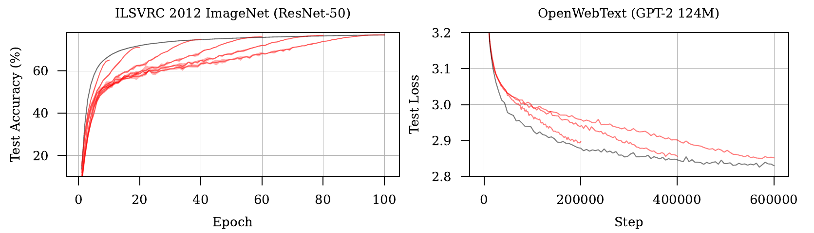
The red lines are several cosine schedules of different lengths, each at its best only at its own endpoint; connect those endpoints and you get the frontier of training time versus performance. The black line trains just once, yet it hugs this frontier at every point in time, and on the GPT-2 side it even sits below the red lines most of the time. In other words, wherever you stop training, the result is about as good as having tuned a cosine schedule for that length in advance.
Nine deep learning tasks
| Task | Metric | Schedule-Free | Best schedule |
|---|---|---|---|
| CIFAR-10 | Accuracy | 96.03 | 95.73 |
| CIFAR-100 | Accuracy | 78.71 | 77.41 |
| SVHN | Accuracy | 98.40 | 98.27 |
| ImageNet | Accuracy | 76.90 | 76.90 |
| IWSLT14 | Loss ↓ | 4.18 | 4.23 |
| fastMRI | SSIM | 0.9112 | 0.9110 |
| Criteo | Accuracy | 0.7915 | 0.7906 |
| MAE fine-tuning | Accuracy | 83.54 | 83.52 |
| GPT-2 124M | Loss ↓ | 2.831 | 2.853 |
Compiled from the legends of Figures 2 and 5 of the paper. The best-schedule column is the authors' tuned cosine or linear-decay schedule; ImageNet uses ResNet-50, and GPT-2 124M is the NanoGPT setup on OpenWebText.
It beats the tuned schedule on seven tasks (with very small margins on fastMRI and Criteo) and ties on ImageNet and MAE fine-tuning. The biggest gap is on CIFAR-100, 1.3 percentage points; on ImageNet both are at 76.90%, while the step-wise schedule gets 76.49%.
A few settings behind these numbers are worth a look.
- Much larger learning rates. On CIFAR-10, Schedule-Free uses a learning rate of 10 against cosine's 0.2; on ImageNet it's 1.5 against 0.05; on NanoGPT, 0.005 against 0.0005. The authors think that being able to use larger learning rates without diverging may be one reason for the faster convergence.
- NanoGPT needs special handling. With , the loss rises rapidly partway through training, and it only stabilizes at 0.98; gradient clipping also has to be turned off, which the authors call crucial.
- The gradient doesn't collapse. On CIFAR-10, SGD with a cosine schedule drives the training loss close to 0 late in training, and the gradient norm collapses to near 0 along with it, after which learning nearly stalls; Schedule-Free doesn't show this. The authors think this may be why it does particularly well on CIFAR and SVHN.
The appendix adds results for Polyak averaging and primal averaging on the same set of tasks, and both fall clearly behind. On ImageNet they reach 72.84% and 69.78%, respectively, and on NanoGPT the Polyak averaging loss diverges outright.
AlgoPerf
The AlgoPerf results in the paper are the authors' own comparison against the NAdamW baseline under the competition rules, over 10 random seeds. The ResNet-50 workload was excluded because neither AdamW nor NAdamW can reach its target. On the remaining 7 workloads, Schedule-Free AdamW is faster on WMT, ViT, fastMRI and OGBG, ties on Conformer and Criteo, and is slightly slower on DeepSpeech. The authors attribute the results on Conformer and DeepSpeech to BatchNorm. Both use BN, and the competition's code framework doesn't make it easy to recompute BN statistics at .
The appendix also lists the single configuration used for self-tuning: learning rate 0.0025, , , weight decay about 0.081, 2% warmup, and averaging weights additionally multiplied by .
The official results are in MLCommons' announcement and in the organizers' later analysis published at ICLR 2025. In self-tuning, Schedule Free AdamW was the only submission to beat the baseline, with average training time about 8% faster, and it was fastest on 4 of the 8 base workloads; compared with the external-tuning baseline, on the 7 workloads both trained successfully, it was still about 10% faster without any tuning. The same team also entered external tuning with a version carrying 5 configurations, taking second place (0.7077) behind Distributed Shampoo's 0.7784; on the 7 workloads where both succeeded, Shampoo was about 24% faster than self-tuning Schedule-Free AdamW.
There was one more twist. The self-tuning prize was never awarded. According to MLCommons' announcement, the prize requirement was not met because several competing submissions involved affiliations that overlapped with the working group chairs.
Sensitivity to momentum
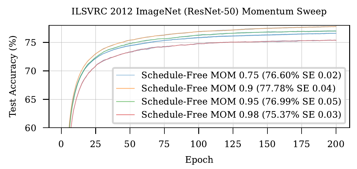
If the best changes with training length, then "no need to know " merely moves the problem from the schedule to the momentum. The authors ran a longer-than-usual 200 epochs on ImageNet and swept four momentum values. Wherever you stop and look, is best. Sensitivity to the learning rate is also similar to that of the cosine schedule; only for very short training (25 epochs or fewer) do somewhat larger learning rates do better.
Other evidence is less rosy, though. NanoGPT itself needed raised to 0.98, and the official README also says may need to go up to 0.95 or 0.98 for particularly long runs. Hägele et al. (NeurIPS 2024) compared Schedule-Free AdamW against a constant learning rate with a final linear cooldown (similar to WSD) on a 210M-parameter language model. With it was clearly worse, and the loss even went up late in training; with it did very well, but both settings were matched or beaten by the cooldown schedule. They also did no further hyperparameter tuning for either side.
Limitations
The authors state plainly in their conclusion that the primary practical limitation is having to re-sweep the learning rate and weight decay, since the best values differ from those used with a schedule. Most of the other points to watch have already come up.
- Warmup is still required. Most of the paper's experiments set warmup to 5% of total training, and the AlgoPerf configuration uses 2%; strictly speaking, the training length still comes in here.
- BN statistics need to be recomputed at ; training and evaluation require switching modes, and so does saving a checkpoint.
- The theory covers only convex problems, and there's no complete theory yet for when large step sizes work.
- is more sensitive in long language-model training runs.
Conclusion
Schedule-Free replaces the learning-rate schedule with three sequences. The base optimizer steps on , is the average of , and the gradient is computed at , between the two. The averaging itself implies a linear-decay schedule whose endpoint keeps moving, so needn't be known in advance; on convex problems, any retains the optimal worst-case rate. Of 9 deep learning tasks it won 7 and tied 2, and it took first place in the AlgoPerf 2024 self-tuning ruleset.
If you want to try it, after swapping in the optimizer, remember to add the matching optimizer.train() and optimizer.eval() next to model.train() and model.eval(), and switch to eval before saving a checkpoint; for models with BN, recompute the statistics at before evaluation. Start with a learning rate 1 to 10 times the scheduled version's (AdamW) or 10 to 50 times (SGD), use 0.9 for first and move toward 0.95 or 0.98 for very long runs, and keep the warmup.
For something called Schedule-Free, line 8 of Algorithm 1 still reads .