Original paper
The Marginal Value of Adaptive Gradient Methods in Machine Learning
- Publication
- NeurIPS 2017Conference
- First submitted to arXiv
- arXiv:1705.08292
Cite this paper · BibTeX
The citation identifies the linked source version. It cites the original paper and its authors.
@misc{optimizersmarginalvalue2017,
  title = {{The Marginal Value of Adaptive Gradient Methods in Machine Learning}},
  author = {Ashia C. Wilson and Rebecca Roelofs and Mitchell Stern and Nathan Srebro and Benjamin Recht},
  year = {2017},
  eprint = {1705.08292},
  archivePrefix = {arXiv},
  url = {https://arxiv.org/abs/1705.08292}
}
"These results suggest that practitioners should reconsider the use of adaptive methods to train neural networks."
That is the last sentence of the paper's abstract.
In May 2017, Adam had been out for just over two years, and the paper's own introduction notes that it was already the default algorithm in many deep learning frameworks. Two claims were going around at the time, that adaptive methods such as AdaGrad, RMSProp, and Adam converge faster, and that they need almost no tuning. Ashia Wilson, Rebecca Roelofs, Mitchell Stern, and Benjamin Recht at Berkeley, together with Nathan Srebro at TTIC, put both claims to the test.
They first constructed a simple classification problem on which SGD's test error is 0 while the adaptive methods get close to half wrong; they then ran experiments on image classification, character-level language modeling, and two kinds of syntactic parsing, and the conclusion every time was that well-tuned SGD wins.
This note first takes apart that constructed example, then looks at the experiments and how they tuned hyperparameters, and finally at how, two years later, another group used the same code to tune the gap away until it could no longer be seen.
Defining the problem
Deep networks usually have far more parameters than training samples, so the solutions that drive the training loss to 0 aren't just one but a whole region. Which one the optimizer ends up at depends on the path it takes, and different solutions that are equally good on the training set can differ a lot on new data.
This paper asks whether adaptive methods and SGD pick different solutions in this situation, and whether the solutions they pick generalize differently.
To compare them, the paper first writes the various methods in a common framework. SGD follows the gradient directly; adaptive methods multiply the gradient by the inverse of a diagonal matrix,
where the choice of determines whether it is AdaGrad, RMSProp, or Adam, with a momentum term added separately. SGD corresponds to and uses the parameter space's original geometry; adaptive methods, based on past gradients, give each coordinate a ruler of its own.
Solving the problem
SGD finds the minimum-norm solution
Start with the simplest case, binary classification by least squares:
When , as soon as there is one solution with zero loss, there are infinitely many.
Every gradient SGD takes has the form , so it lies in the row space of . Starting from and using only linear combinations of gradients and past iterates, SGD can never leave this space. Within the row space there is only one solution satisfying , namely , which happens to be the solution with the smallest norm of them all, and also the one with the largest margin.
So SGD, momentum, mini-batch SGD, Nesterov, and even the conjugate gradient method all end up at the same point. The paper calls the fact that gradient descent naturally finds the maximum-margin solution "a pleasant surprise."
Adaptive methods find the sign solution
The denominator of an adaptive method differs from coordinate to coordinate, so the row-space constraint no longer applies. In general it is hard to work out where it will converge, so the paper picks a special case it can compute (Lemma 3.1):
If there exists a scalar such that , then starting from , AdaGrad, Adam, and RMSProp all converge to the unique solution .
The idea of the proof is straightforward. While is proportional to , the gradient is proportional to and the denominator is proportional to ; divide one by the other, and every coordinate's update has the same magnitude, differing only in sign. So after every step, is still proportional to , and induction gives the result.
Put differently, in this special case, adaptive methods treat every feature as equally important, and every weight has the same absolute value. In the paper's words, they converge to solutions with a small norm, while SGD converges to solutions with a small norm.
Constructing data that trips it up
Next, the paper designs a dataset that turns this difference into test error.
Each sample's label is with probability and otherwise. The feature vectors are long, and the first three dimensions are treated separately from the rest:
- Dimension 1 is the label itself, ;
- Dimensions 2 and 3 are always 1;
- The rest give each sample a stretch of features that belong to it alone, 1 feature for a positive example and 5 for a negative one, all with value 1.
Only dimension 1 is actually useful; dimensions 2 and 3 are constants, and each of the remaining features appears in only one sample. On the training set they look highly discriminative, since each one can "recognize" a particular sample, but they are useless for new samples.
This dataset satisfies the condition of Lemma 3.1, with . We worked it through with 10 training samples (6 positive, 4 negative). Starting from , both gradient descent and Adam drive the training loss to 0, and the learned weights are as follows:
| Feature | SGD | Adam |
|---|---|---|
| Dimension 1 (label) | 0.756 | 0.25 |
| Dimensions 2 and 3 (constant) | 0.087 | 0.25 |
| Positive example's own feature | 0.070 | 0.25 |
| Negative example's own features | −0.084 | −0.25 |
Computed for this note. The SGD column is the minimum-norm solution; gradient descent run to convergence matches the closed-form solution. The Adam column uses the default values and a learning rate of for twenty thousand iterations; AdaGrad gives the same weights.
SGD puts most of the weight on dimension 1. Adam gives every feature the same weight, with the sign following each feature's relationship to the label on the training set.
Now a new sample arrives. Its own features are brand new and never appeared during training, so the only overlap with is in the first three dimensions:
- SGD: the score is . A positive example scores and a negative one , so both are classified correctly.
- Adam: the score is . A positive example scores and a negative one , so both are classified as positive.
On this dataset, adaptive methods label every unseen sample as positive, so their test error is the fraction of negatives, . The closer is to , the closer the error gets to one half, while SGD's error is 0. The appendix also gives a version that samples from a fixed distribution, with the same conclusion.
The dimension in this example doesn't actually need to be infinite; the paper says dimensions are enough, and deep networks often have 25 times as many parameters as samples, or more. The authors' reading is that real data also often has a few frequently occurring, genuinely useful features alongside a large number of sparse ones; on a finite training set, the sparse features look very good at telling samples apart, but that is just overfitting.
Going by the mechanism in Lemma 3.1 (this explanation is ours), an adaptive method's denominator comes from each coordinate's own past gradients, so sparse features that rarely appear have small denominators and take relatively large steps, and they end up pushed to the same weight as the genuinely useful features, which amplifies exactly this problem.
The construction has its prerequisites. It requires starting from and data with the special structure , and the analysis drops the in the denominator. What it proves is that adaptive methods can generalize very poorly; whether that happens in neural networks is a question for the experiments.
Discussion
Experimental setup
The paper compares two non-adaptive methods (SGD and heavy-ball with momentum fixed at 0.9, HB below) with three adaptive methods (AdaGrad, RMSProp, Adam), plus one more line for Adam with all default settings. All four tasks use publicly available code, with the architectures and preprocessing left as unchanged as possible:
| Task | Model | Data |
|---|---|---|
| Image classification | VGG+BN+Dropout | CIFAR-10 |
| Character-level language model | 2-layer LSTM | War and Peace |
| Discriminative parsing | 2-layer LSTM + feedforward | Penn Treebank |
| Generative parsing | 3-layer LSTM | Penn Treebank |
Compiled from Table 2 of the paper. The four codebases use three frameworks, Torch, DyNet, and TensorFlow; the first two tasks both use Torch.
Syntactic parsing breaks a sentence down into a tree of nested clauses, phrases, and words. The discriminative approach turns tree building into predicting a sequence of actions and is measured by F1; the generative approach writes the tree as a depth-first traversal sequence and scores it like a language model, measured by perplexity.
Each setting is run 5 times from random initializations. The number of training epochs is fixed in advance; for tasks with a validation set, the setting with the best validation result within the budget is selected, while CIFAR-10, which has no separate validation split, instead selects the setting with the lowest training loss.
How they tuned
The authors found that the two hyperparameters with the most impact were the initial learning rate and the decay scheme, so they tuned only those two and left everything else at each framework's defaults.
The learning rate takes 5 points on a log scale. If the best point falls at the edge, more points are added beyond it until the best value is in the middle; for example, if 2, 1, 0.5, 0.25, and 0.125 are tried and 2 is best, 4 is tried next, and if 4 is better, 8 after that. There are two decay schemes:
- dev-decay: track the best validation result so far, and whenever an epoch fails to improve on it, multiply the learning rate by ;
- fixed-decay: multiply by every epochs.
The authors recommend dev-decay when a validation set is available, since it has fewer hyperparameters and does no worse than fixed-decay. The appendix lists the learning rates tried for each method. On CIFAR-10, for example, SGD's best was 0.5 and Adam's best was 0.0003, less than a third of the default 0.001.
CIFAR-10
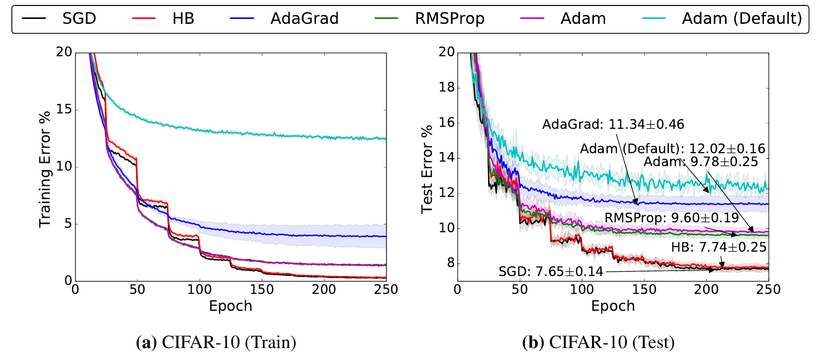
The model is the VGG+BN+Dropout from the Torch blog, whose original test error was 7.55%. The right panel marks each method's best test error: SGD at , RMSProp, the best of the adaptive methods, at , tuned Adam at , and default Adam at .
Following the curves over time is more revealing. For the first 50 epochs, the adaptive methods are clearly ahead in training error, while their test error is on par with SGD and HB. From about epoch 50 on, the adaptive methods still have lower training error, but SGD and HB have already pulled ahead in test error; by epoch 100, SGD and HB are winning on both training and test. In the left panel, SGD and HB drop a step every 25 epochs, which is the learning-rate decay; when Choi et al. reran this experiment two years later, the setting they recorded was multiplying the learning rate by 0.5 every 25 epochs. The adaptive methods' curves are much flatter at the same points.
The authors also tried larger learning rates for the adaptive methods. That did help over the first 50 epochs, but they stalled even worse later, and no decay scheme could rescue them.
Three language tasks
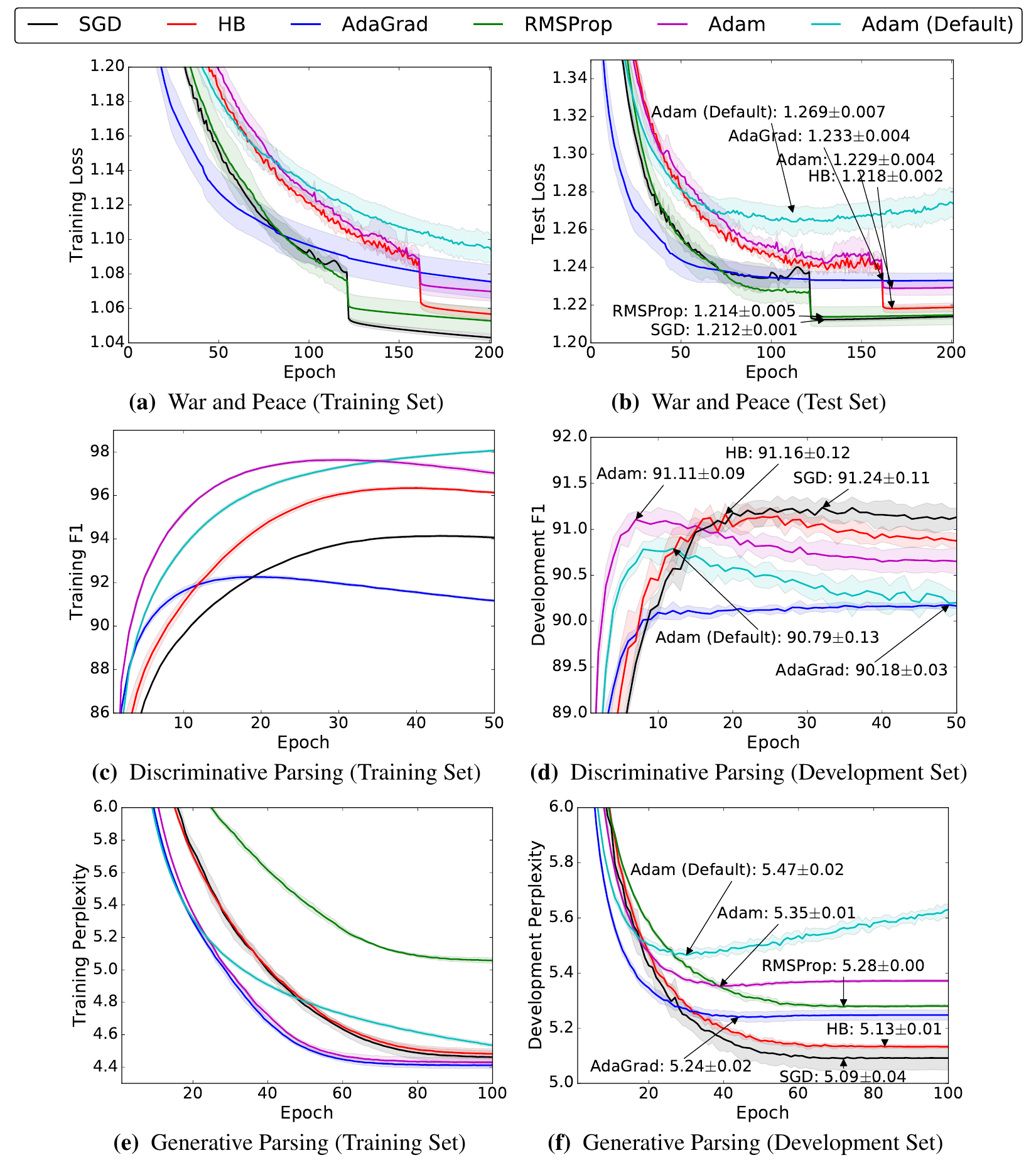
In each row, the left is the training set and the right is the validation or test set, with each method's best value marked.
- Character-level language model (first row). Trained with torch-rnn on the full text of War and Peace for 200 epochs. SGD has the lowest test loss, ; RMSProp follows closely at , which the authors point out shows that adaptive methods can find solutions that generalize well. The fixed-decay search also found that for every method except AdaGrad, the best setting divided the learning rate by 10 just once, 60% or 80% of the way through training.
- Discriminative parsing (second row). The parser of Cross and Huang, trained on the Penn Treebank for 50 epochs, with dev-decay's ; DyNet at the time had no RMSProp. SGD has the best validation F1, 91.24, with HB and Adam close behind. Adam needs only 6 epochs to reach its best of 91.11, while SGD takes 18 epochs to match that number and 31 epochs to reach 91.24. After that, Adam keeps improving on the training set while its validation score drops.
- Generative parsing (third row). The model of Choe and Charniak, with the LSTM hidden dimension reduced from 1500 to 500 and dropout from 0.7 to 0.5 to save compute, trained for 100 epochs. SGD has the best validation perplexity, 5.09; Adam's training curve is among the best, yet its validation perplexity, 5.35, is the worst among the tuned methods.
Across the four tasks, the findings come down to four points:
- The solutions found by adaptive methods generalize worse than those found by non-adaptive methods.
- Even when their training loss is just as low or lower, adaptive methods still do worse on validation or test.
- Adaptive methods make fast progress on the training set at first, but their validation performance soon stalls.
- Tuning the learning rate and decay improves Adam noticeably on every task. Default Adam is at or near the bottom in all four plots, so the claim that "Adam needs no tuning" doesn't hold up.
In their conclusion, the authors say they aren't sure why Adam remains so popular. Their guess, after talking with other researchers, is that Adam is especially popular for GANs and for Q-learning with function approximation, and since neither of these is, strictly speaking, solving an optimization problem, Adam's dynamics may happen to suit them.
Comparing again with tuned
Two years later, Dami Choi, Christopher Shallue, George Dahl, and colleagues from the University of Toronto and Google Brain responded to this paper in "On Empirical Comparisons of Optimizers for Deep Learning."
Their starting point is the inclusion relationships between optimizers. Set momentum to 0 and you get SGD, so the best-tuned momentum can't lose to the best-tuned SGD. Adam can also mimic momentum. Set to 0 and make very large, and the denominator is essentially the constant ; pair that with a learning-rate schedule that cancels out the bias correction, and Adam's update becomes SGD with momentum. So as long as every hyperparameter is tuned, Adam shouldn't do worse than momentum.
Wilson et al. tuned only the learning rate and the decay, leaving at each framework's default, and the analysis of the constructed example also dropped . Choi et al. reran Wilson et al.'s publicly released CIFAR-10 code:
- Sweeping only the learning rate, as in the original, reproduced the result that RMSProp and Adam do worse;
- Using random search to also tune the momentum-related parameters and made the test errors of SGD, momentum, RMSProp, and Adam nearly identical;
- Switching to their own code and searching over learning-rate schedules, the four also landed within the margin of error.
They also noted that Wilson et al. selected settings on CIFAR-10 by training loss; switching to selection on a validation set didn't change the conclusion. turned out to matter more than expected, and across four tasks the best they found spanned 10 orders of magnitude.
Choi et al. also offered their own explanation of how the two papers' conclusions fit together. If "Adam with default " and "Adam with tuned " are treated as two different optimizers, there's no contradiction. It's worth thinking one step further here. With a large , Adam's denominator is also less adaptive, and the optimizer gets closer and closer to momentum SGD. When Choi et al. tuned for Adam on Wilson's code, the final search range was to , several orders of magnitude larger than the gradients, so the denominator was essentially constant. Read together, then, the two papers say that adaptive updates under default settings can indeed generalize worse, and that part of what gets Adam to match SGD is a set of hyperparameters that makes it less adaptive.
Other responses
Around the same time, several other lines of work approached this gap from different angles.
- Get weight decay right. In November 2017, Loshchilov and Hutter cited this paper and argued that a major reason for Adam's poor generalization is that L2 regularization doesn't do its job inside Adam, and proposed AdamW.
- Switch to SGD later on. Keskar and Socher's SWATS trains with Adam first and switches to SGD when a certain condition is triggered; AdaBound clamps each parameter's learning rate in Adam between lower and upper bounds that gradually tighten, transitioning smoothly from Adam to SGD.
- Large-scale re-comparison. Schmidt et al. compared 15 optimizers using more than fifty thousand training runs and found that none clearly won on every task, with Adam still a strong choice.
The other development, pointing the opposite way, is the Transformer. Choi et al. did see a clear ranking on a Transformer language model on LM1B, where Adam needed only 60% of the steps momentum needed to reach the target error, and only 25% of SGD's to reach the same final result. Zhang et al. argued in 2019 that the heavy-tailed distribution of gradient noise in attention models is one reason SGD performs poorly; Kunstner et al. in 2023 grew the batch all the way to the full dataset and found that as noise decreased, Adam improved more than SGD, so the gap didn't shrink. This paper's experiments stop at 2017-era CNNs and LSTMs, and its conclusions can't be directly extrapolated to models like these.
Conclusion
Using a constructed example, this paper proves that on over-parameterized problems, adaptive methods and SGD can end up at different solutions; under a particular data structure, the solution an adaptive method learns can misclassify half of the new data, while SGD gets everything right. In all four experiments, with only the learning rate and decay tuned, SGD and HB had better test results, and default Adam lagged clearly behind. Two years later, Choi et al. reran the same code with and other hyperparameters tuned as well, and the gap on CIFAR-10 disappeared.
When you read a paper comparing optimizers, look for the section on tuning first: which hyperparameters were tuned, how many values each one got, and how the settings were selected. The same goes for your own comparisons. For Adam, tune at least the learning rate, the learning-rate schedule, and , and, as this paper's appendix does, write down the grid you actually tried for each method.
When Choi et al. trained ResNet-50 on ImageNet, their best NAdam setting had an of 9475. A constant that was only ever supposed to keep us from dividing by zero didn't even have a place in Wilson et al.'s grid.