Original paper
Fantastic Pretraining Optimizers and Where to Find Them
- Publication
- ICLR 2026Conference
- First submitted to arXiv
- arXiv:2509.02046
Cite this paper · BibTeX
The citation identifies the linked source version. It cites the original paper and its authors.
@misc{optimizersfantasticoptimizers2025,
  title = {{Fantastic Pretraining Optimizers and Where to Find Them}},
  author = {Kaiyue Wen and David Hall and Tengyu Ma and Percy Liang},
  year = {2025},
  eprint = {2509.02046},
  archivePrefix = {arXiv},
  url = {https://arxiv.org/abs/2509.02046}
}
Take a 130M-parameter language model and train it with AdamW using the GPT-3 paper's recipe, with a peak learning rate of 6e-4. Now change just one number, the learning rate, to 8e-3, and leave every other setting alone. It reaches the same loss in half the steps.
This experiment is in the paper's first figure. That AdamW curve with the GPT-3 recipe is exactly the baseline used by papers on new optimizers such as Sophia, MARS and Cautious, and most of the speedups they claim are 2×. The large-scale version of Muon claims about 2×, SOAP claims 1.4×, and DION even reports 3×.
If tuning the baseline's learning rate alone gives 2×, how much faster are these optimizers really? Kaiyue Wen, David Hall, Tengyu Ma and Percy Liang at Stanford put 11 optimizers through the same pipeline, tuning each from scratch, and compared them all the way from 130M to 1.2B parameters.
The paper's title riffs on the film Fantastic Beasts and Where to Find Them. This note looks at how they designed a fair comparison, what speedups they measured, and how their results differ from several large-scale evaluations from the same period and after.
Defining the problem
The authors argue that new optimizers have been slow to replace AdamW because of how they are evaluated, and they see two main problems.
The first is unequal tuning. Authors of a new method usually tune their own optimizer carefully, while the baseline keeps an old recipe, or all optimizers share a single learning rate and weight decay.
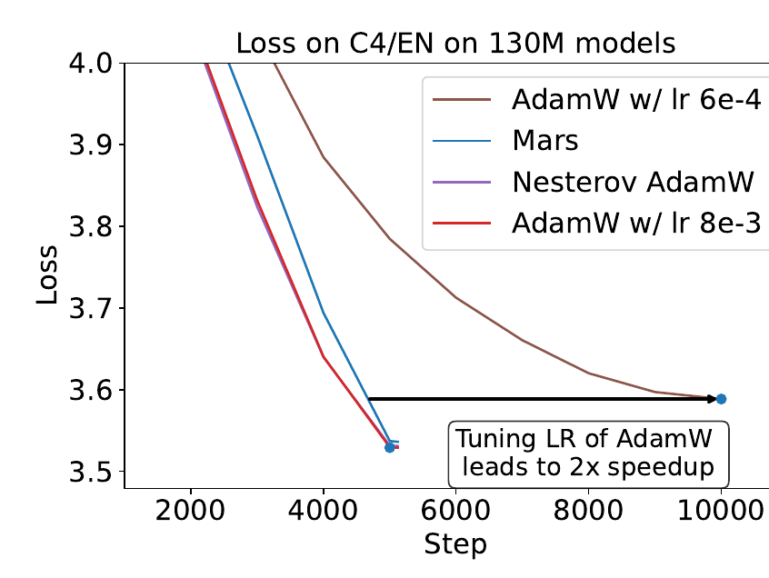
The brown line is AdamW at a learning rate of 6e-4 and the red line at 8e-3. The red line gets down to the brown line's final loss at step 10,000 in under 5,000 steps, and ends even lower, at about 3.53. MARS (blue) and Nesterov AdamW (purple) are also plotted, and both end very close to the tuned red line. With the brown line as the baseline, MARS looks like a 2× speedup; switch to the red line, and the gap is much smaller.
Shared hyperparameters aren't fair either. Even optimizers that look alike can have very different best hyperparameters. For Lion, the paper's sweeps find the best weight decay at about 0.6, against about 0.1 for AdamW; if the two share one value, one of them is bound to lose out.
The second is evaluation setups that are too narrow. Most papers compare only near 1× Chinchilla, on one or two model sizes, and some even compare intermediate checkpoints. 1× Chinchilla is the compute-optimal ratio derived in the Chinchilla paper, about 20 tokens per parameter. Real large models range from 1× to over 50×, and a method that wins at 1× won't necessarily still win where data is plentiful.
These are the two things this paper sets out to answer. How do you make sure every optimizer is tuned close to its best? And what are the speedups across different model sizes and data amounts?
Solving the problem
The testbed
The data follows OLMo 2, mixing DCLM-baseline (3.8T tokens), StarCoder V2 (0.25T) and ProofPile 2 (55B), with the Llama 3 tokenizer. All models use the Llama architecture with 32 layers and a sequence length of 4,096, varying only the width:
| Model | Hidden dimension | Feed-forward dimension | Attention heads |
|---|---|---|---|
| 130M | 512 | 2,048 | 8 |
| 300M | 768 | 3,072 | 12 |
| 520M | 1,024 | 4,096 | 16 |
| 1.2B | 1,536 | 6,144 | 24 |
Compiled from Table 2 of the paper.
Data amounts are expressed as Chinchilla multiples, 1×, 2×, 4× and 8× (with 1× being 20 times the non-embedding parameter count). The main metric is validation loss on the English subset of C4, with more than ten downstream accuracies, such as HellaSwag and ARC, tracked as well. The experiments run in JAX on 128 TPU v5 lite chips, which the authors estimate is roughly equivalent to 12 H100s.
The unit of comparison is how many tokens it takes to reach the same loss, leaving out the extra compute time per step. The authors' reasoning is that both SOAP and Kimi's Muon paper show that, when implemented well, matrix-based optimizers can keep the per-step overhead under 10%.
The 11 optimizers fall into five groups:
- Baseline: AdamW
- AdamW variants that reduce update variance: NAdamW (Nesterov momentum), MARS, Cautious
- Memory-efficient: Lion, Adam-mini
- Matrix-based: Muon, Scion, Kron (PSGD), SOAP
- Approximate Hessian: Sophia (results in the appendix)
Scalar-based and matrix-based optimizers differ in how the preconditioner acts. Scalar-based ones such as AdamW, Lion and MARS multiply each parameter by its own scalar; matrix-based ones such as Muon, SOAP and Kron treat the whole weight matrix as one unit and process the gradient with matrix multiplications.
Three-phase tuning
A full search over every combination is too expensive, so the authors work in three phases.
Phase one is coordinate descent. Each hyperparameter has a discrete set of candidate values; for AdamW, these cover the learning rate, weight decay, warmup steps, , , , the gradient-clipping threshold and the batch size. The starting point is the setting recommended by the method's original paper. Each pass fixes the other hyperparameters and sweeps just one, switching to a new value if it improves the validation loss by more than ; passes repeat until no single hyperparameter gives a significant improvement. This is done once for each of 6 settings: 1× at 130M, 300M and 520M, plus 2×, 4× and 8× at 130M.
The paper walks through an example for AdamW. The initial setting is a learning rate of 0.008, weight decay 0.1, 1,000 warmup steps and a batch of 256 sequences, with a loss of 3.298; the first pass changes warmup to 2,000 steps, lowering the loss to 3.282; the second changes the batch to 128 sequences, lowering it to 3.263; finally, the gradient-clipping threshold changes to 2, the loss stays at 3.263, and the sweep ends.
Phase two tunes only the hyperparameters that change with scale. The authors observed two things. Many hyperparameters barely affect the loss as long as they are near their best value; and for the ones that do matter, the best value mostly doesn't change with scale either.
So they count any setting whose loss is within of the best as “near-optimal.” If some value of a hyperparameter is near-optimal in every setting, that hyperparameter is scale-insensitive and gets fixed; otherwise it is scale-sensitive and is carried into phase two for further tuning.
In the end, each optimizer has only a few hyperparameters to retune. For AdamW they are the learning rate, warmup, weight decay and batch size; for Lion, the learning rate and ; for Muon and Kron, only the learning rate. Phase two reruns on 6 settings, 2×, 4× and 8× at 300M and 520M, which together with phase one makes 12 settings.
Phase three extrapolates the pattern. For each hyperparameter that needs retuning, the best values across the 12 settings are fit with
where is the parameter count and the token count. To validate this, the authors redid a full phase one for AdamW at 1.2B, 1×; the hyperparameters predicted by the fit give a loss within of the best actually found. They then used these predictions for two larger case studies, one with the 1.2B model from 1× to 8×, the other with 130M and 300M models trained all the way to 16×.
How the best values shift with scale can be seen directly in the appendix tables. For AdamW at 130M, 1×, the best learning rate is 0.008, with weight decay 0.1 and a batch of 128 sequences; at 1.2B, 1×, it becomes a learning rate of 0.002, weight decay 0.2 and a batch of 256. Muon's learning rate for the matrix parameters drops from 0.016 to 0.004 (at 1.2B, 1×, switching to 0.008 gives a slightly lower loss still). The model grows about 9 times and the learning rate shrinks by 2 to 4 times, so if you use the learning rate tuned at 130M directly at 1.2B, the baseline loses out.
How speedup is measured
Speedup is converted through token counts. For each model size, a curve is first fit to AdamW's four losses at 1×, 2×, 4× and 8×:
If an optimizer reaches loss with tokens, inverting AdamW's curve gives the tokens AdamW needs to reach the same . The speedup is .
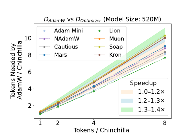
To read this plot, look at how far each line sits from the diagonal. An optimizer exactly as fast as AdamW would land on ; the higher a point, the more tokens AdamW has to read to catch up. At 520M, the solid matrix-based lines fall roughly within the 1.2-to-1.4× bands, and the more data there is, the more clearly they bend upward.
Discussion
Main results: at most 1.4×, and less at larger scale
Across three model sizes and four data amounts, four patterns emerge.
- No method reaches 2×. Against a well-tuned AdamW, the best is about 1.4×. SOAP is one of the few papers that seriously tuned its own baseline, and its claimed 1.4× is the closest to what was measured here, which is actually 1.2 to 1.3× at 300M and 520M.
- Matrix-based beats scalar-based. At every model size, Muon, SOAP, Kron and Scion all beat the scalar-based optimizers. Muon is the best at 1×; by 8×, SOAP and Kron have caught up and overtaken it. The speedup of matrix-based optimizers grows with the amount of data and shrinks as models get larger.
- Once tuned, scalar-based optimizers are all about the same as AdamW, with average speedups under 1.2×. The variance-reducing variants NAdamW, MARS and Cautious edge out AdamW slightly.
- The memory-efficient Lion and Adam-mini track AdamW closely, at most 5% slower and occasionally slightly faster. As models grow, Lion falls further and further behind, while Adam-mini actually closes in.
The best loss for each setting in the appendix shows directly how small the gaps are. A few cells:
| Optimizer | 130M, 1× | 520M, 8× | 1.2B, 8× |
|---|---|---|---|
| AdamW | 3.529 | 2.913 | 2.752 |
| NAdamW | 3.531 | 2.907 | 2.749 |
| Lion | 3.552 | 2.915 | — |
| Muon | 3.464 | 2.906 | 2.748 |
| SOAP | 3.483 | 2.899 | 2.749 |
Compiled for this note from the best-setting rows for each configuration in Appendices C, D and E of the paper; C4/EN validation loss, lower is better. Only four optimizers were run at 1.2B.
At 130M, 1×, Muon is 0.065 below AdamW, the largest gap in the table. At 1.2B, 8×, the four optimizers are packed within 0.004 of each other.
1.2B: down to 1.1×
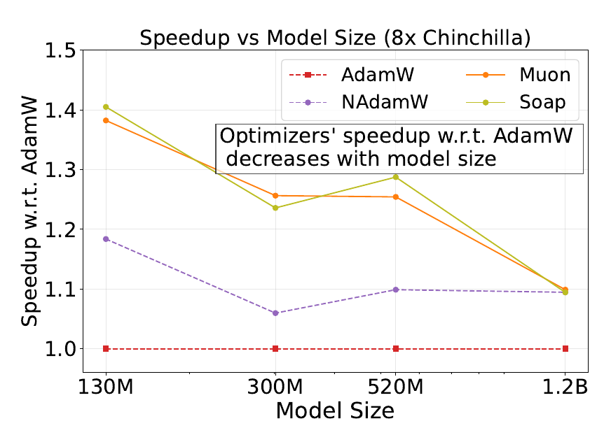
This plot holds the data at 8× Chinchilla and shows how speedup changes with model size. SOAP and Muon are both close to 1.4× at 130M, but by 1.2B only about 1.1× is left, almost the same as NAdamW.
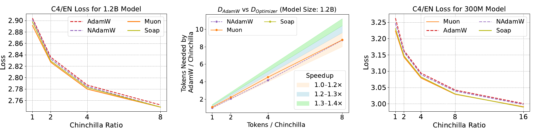
The left plot is the 1.2B loss. NAdamW, Muon and SOAP are still faster than AdamW, but there is almost no gap among the three; converted to speedup in the middle plot, it comes to about 1.1×. Downstream evaluations show no difference either; at 8× (193B tokens), the ten-task average is 67.15 for AdamW, 66.70 for NAdamW and 66.98 for Muon.
Using 16 training runs, the authors fit scaling laws for AdamW and Muon, and predict that at 7B, 1×, Muon's loss would actually be higher than AdamW's. Computing from the coefficients in the appendix, at 7B, 1× AdamW comes to 2.5706 and Muon to 2.5729, a difference of 0.002, smaller than the 0.005 RMS error of Muon's own fit. This prediction extrapolates 6 times beyond the fitted range; what it supports is that Muon's advantage shrinks to nothing visible along this line, while which of the two would win is still an open question.
The right plot extends to 16× Chinchilla. At 8×, SOAP had already overtaken Muon at 130M and 520M; the authors checked again by training 300M all the way to 16×, and SOAP still came out ahead, as it did at 130M. They speculate that the second-order momentum SOAP and Kron keep becomes more useful when data is plentiful. In the appendix tables, though, the best losses at 300M, 16× are 2.990 for SOAP and 2.991 for Muon, just 0.001 apart, which is smaller than the 0.003 threshold their own coordinate descent uses to count something as an improvement. A safer reading of this part is that once the data amount goes up, Muon's earlier lead disappears.
Early curves can mislead
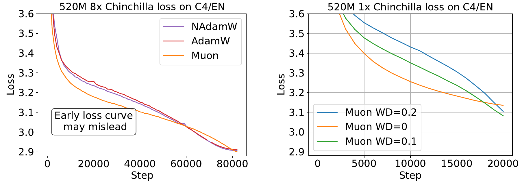
The left plot shows the full training curves at 520M, 8×. Muon leads by a wide margin in the first half; stop and compare at step 30,000, and it looks much faster. Once the learning rate starts decaying sharply, AdamW and NAdamW catch up, the three lines cross around step 60,000, and they finish almost level.
The right plot is the same optimizer with three different weight decays. Muon without weight decay is the fastest early on but then stalls, finishing the worst of the three; weight decay 0.1 ends the best.
So the authors recommend comparing only final checkpoints. Here they single out Kimi's Muon paper, whose comparison of Muon and AdamW MoE models used exactly that kind of intermediate checkpoint, taken before the learning rate had finished decaying.
The same section has two more observations.
- A single hyperparameter can flip the ranking. At 520M, 8×, setting SOAP's learning rate to twice its best value almost wipes out its lead over MARS. The authors collected every run that changes only one hyperparameter and stays within 0.02 of the best loss, and the distributions for Muon, SOAP and MARS overlap one another. Without systematic sweeps, the ranking can be almost arbitrary.
- The best weight decay depends on the optimizer. As mentioned earlier, Lion's is about 0.6; Kron's is about 0.5, which is key to it beating AdamW.
Where the earlier 2× claims came from
Appendix G goes through the setups of earlier papers one by one to find why their speedups were overestimated.
- Sophia (2×): the peak learning rate was below 6e-4. One reason is that the Levanter data loading used at the time didn't fully shuffle the data; when reproducing it, the authors found that a large learning rate only works stably with full shuffling. In their setup, Sophia shows no significant speedup below 0.5B.
- MARS (2×): a baseline similar to Sophia's. A figure in the first version of the MARS paper already shows AdamW improving substantially when its learning rate is raised to 3e-3.
- Muon (2×): about 1.3× on the NanoGPT speedrun. Kimi measured 2×, but their AdamW learning rate was on the low side, only 8e-4 to 9e-4 for 400M to 1.5B, and the MoE comparison was taken before the learning rate had fully decayed. Essential AI's independent study measured a token efficiency of 1.1 to 1.2×.
- SWAN and DION (2 to 3×): compared in the regime below 1× Chinchilla, where speedups are larger to begin with; the communication cost that DION is mainly about isn't counted in this paper.
- SPlus (2×): used a constant learning rate with no decay, which isn't the usual pretraining setup.
Another evaluation from the same time
One day before Fantastic, Semenov, Pagliardini and Jaggi at EPFL posted Benchmarking Optimizers for Large Language Model Pretraining on arXiv. They trained about 2,900 models using about 30,000 GPU hours, likewise comparing 11 methods, on models from 124M to 720M plus a 520M MoE; the data is FineWeb, with sequences only 512 tokens long and batches ranging from 16 thousand to 2 million tokens.
The two studies agree on a good deal, for example that weight decay shouldn't be 0, that the learning rate should decay low enough, and that variance-reducing AdamW variants like MARS do help. The biggest disagreement is over matrix-based optimizers. Semenov et al. found AdEMAMix and MARS beating Muon, with both far ahead at 720M with 1 million tokens per batch; Fantastic found Muon clearly beating MARS.
Fantastic analyzes the reasons itself in its related-work section.
- Batch size: Semenov et al.'s most carefully tuned experiments, at 124M, use only 16 thousand and 130 thousand tokens per batch, while the batches Fantastic's tuning arrived at are all at least about 400 thousand tokens. MARS and AdEMAMix average gradients to reduce noise, which pays off in the noise-dominated small-batch regime; once batches get large, that advantage shrinks.
- Hardware: EPFL appears to use mainly 1 to 8 H100s, where small batches are more economical; Fantastic uses 128 TPUs, which need large batches to put their parallelism to full use.
- Tuning: at around 520M, the best learning rates Fantastic found are 4e-3 to 8e-3, while EPFL used 1e-3 to 2e-3, some of them carried over from smaller models without retuning; Fantastic also tunes the learning rates for Muon's embedding layer and matrix weights separately.
The two studies also echo each other. EPFL found that Lion and Signum improve markedly with larger batches but fall behind again on larger models, and that Muon with weight decay is stable in every setting, while the original Muon degrades as models grow.
Larger scales
The paper itself lists the 1.2B ceiling as a limitation. In July 2026, NVIDIA's SOAP, Muon, and Beyond: Pushing LLM Pretraining Scales pushed the comparison to tens of billions of parameters.
Their setup is very different from Fantastic's.
- Models and data: an 8B dense model, plus MoEs with 30B total and 3B activated parameters and with 72B total and 8B activated parameters, trained on 1 to 3 trillion tokens.
- Batch size: a baseline of about 25 million tokens per batch, scaled up to 2×, 3× and 4×; the abstract mentions up to about 100 million tokens.
- Tuning: AdamW uses Nemotron's original production recipe; the learning rates for Muon and SOAP are mostly converted through Kimi's update-RMS matching, and the learning rate is adjusted by a square-root rule when the batch grows, without the one-by-one sweeps Fantastic does.
Muon and SOAP consistently beat AdamW, with the gap widest at large batch sizes. As the batch grows, AdamW degrades while Muon stays stable. On the 30B MoE at the same batch size, Muon's downstream scores are mostly level or higher, for example 58.19 vs 54.45 on MMLU-Pro and 82.52 vs 79.65 on the math average; on the 72B MoE, Muon at 2× batch against AdamW at 1× batch is 4.5 higher on the code average but 3.2 lower on the math average. Once its instability at large batch sizes is fixed, SOAP reaches a slightly lower loss than Muon, and they recommend it when memory allows.
These two sets of results can coexist. Fantastic measures token efficiency after thorough tuning, at batch sizes where AdamW is comfortable (about 0.5 to 1 million tokens); NVIDIA measures who still holds up when the batch is pushed far beyond AdamW's critical batch size. Essential AI saw the same pattern from 100M to 4B, with Muon using 10% to 15% fewer tokens to reach the same loss and keeping or widening that advantage as batches grew.
Other observations and limitations
All optimizers share a few more patterns. With weight decay, the parameter norm rises and then falls along with the learning-rate schedule; the gradient norm rises during learning-rate decay, yet the loss doesn't get worse with it; and each optimizer's training and validation losses move together, with none generalizing noticeably better.
On limitations, the authors state plainly that the largest model is 1.2B. Other conditions are worth keeping in mind too. The paper compares only token efficiency, leaving out wall-clock time and communication; it uses a single data recipe and the dense Llama architecture; and all batches are hundreds of thousands of tokens or more.
Conclusion
This paper uses three-phase tuning to bring each of 11 optimizers close to its best, then converts the results into token efficiency from 130M to 1.2B and from 1× to 8× Chinchilla. Once everything is tuned, the fastest matrix-based optimizers are about 1.3 to 1.4× on small models and only about 1.1× at 1.2B, while scalar-based ones are about the same as AdamW. The earlier 2× claims mostly came from weak baselines and intermediate checkpoints.
When reading an optimizer paper, first check whether AdamW's learning rate was swept, whether the comparison uses checkpoints from the end of training, and how many model sizes and data amounts the experiments span. Before switching optimizers yourself, sweep AdamW's learning rate, weight decay and warmup first; if you're starting from a low learning rate like the GPT-3 recipe's, that step alone could save half your steps.
As for where to find the beasts, judging by NVIDIA's 2026 results, they're probably somewhere above 25 million tokens per batch.