Original paper
Sharpness-Aware Minimization for Efficiently Improving Generalization
- Publication
- ICLR 2021Conference
- First submitted to arXiv
- arXiv:2010.01412
Cite this paper · BibTeX
The citation identifies the linked source version. It cites the original paper and its authors.
@misc{optimizerssam2020,
  title = {{Sharpness-Aware Minimization for Efficiently Improving Generalization}},
  author = {Pierre Foret and Ariel Kleiner and Hossein Mobahi and Behnam Neyshabur},
  year = {2020},
  eprint = {2010.01412},
  archivePrefix = {arXiv},
  url = {https://arxiv.org/abs/2010.01412}
}
Train a ResNet with SGD, and it ends up in a sharp, narrow hole; train the same ResNet another way, and it settles at the bottom of a wide bowl. Both points have very low training loss, and the model has exactly as many parameters in both.
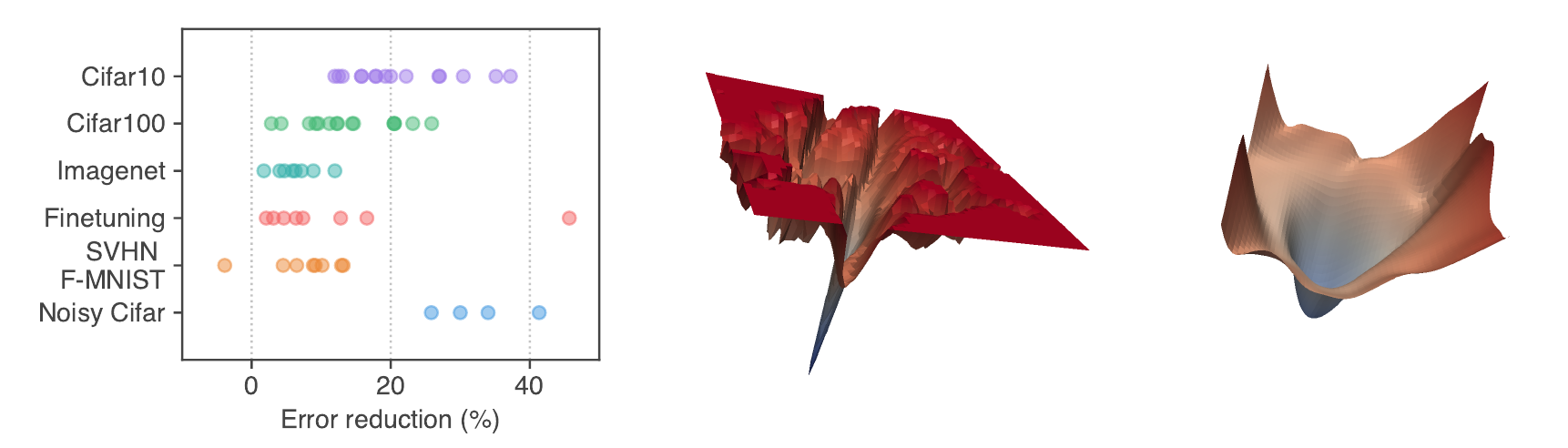
The two landscapes in the middle and on the right are the picture Pierre Foret, Ariel Kleiner and Hossein Mobahi of Google Research and Behnam Neyshabur of Blueshift, part of Alphabet, put on the first page of their paper (the model is a ResNet-56 with its residual connections removed). The left panel is their track record. Across dozens of settings, switching to SAM lowers the error rate almost every time, with reductions ranging from a few percent to over 40%.
The claim that flat minima generalize better is old, going back at least to the 1990s. This paper's approach is that if you want flatness, you write it straight into the objective, and make it cheap enough to train ImageNet with.
Defining the problem
Modern neural networks have enough parameters to memorize the entire training set. The training loss has many minima that are almost equally low, yet they perform very differently on the test set, and which one you end up in depends largely on the optimizer and its settings.
There is already plenty of research on how sharpness relates to generalization. Keskar et al. observed that large-batch training tends to stop at sharp minima and generalize worse; in 2019, Jiang et al. compared 40 complexity measures and found that the sharpness-based ones correlate best with the generalization gap.
The problem is that most previously proposed sharpness measures are hard to compute and even harder to differentiate. Entropy-SGD regularizes local entropy instead; SWA averages the weights from late in training and can land in a flatter spot, but it doesn't minimize sharpness directly. The authors want a procedure that optimizes sharpness directly and scales to large models.
Solving the problem
From a generalization bound to min-max
The starting point is a PAC-Bayes generalization bound (an informal version of Theorem 1). For any , with high probability,
is the population loss, the training loss, and an increasing function. Split the right-hand side:
The bracketed term measures how much the loss can rise at most within a ball of radius around , which is the sharpness. Replacing with ordinary L2 regularization , the authors get SAM's objective:
Instead of looking for a point whose own loss is low, it looks for a point whose whole neighborhood has low loss.
First-order approximation:
The inner maximization can't be solved exactly. The authors take a first-order Taylor expansion of around :
Maximizing an inner product over a norm ball is the classic dual-norm problem. With , the solution is the gradient rescaled to length :
In other words, walk a distance uphill along the gradient. The appendix also tries (), which works worse than ; a perturbation of the same length in a random direction also does worse than one along the gradient.
Next comes the gradient of . is itself a function of , so the chain rule brings in a term , which hides a Hessian:
The second term could be computed with a Hessian-vector product, but the authors drop it to save compute, leaving the gradient
Take the gradient at the perturbed point , then use it to update the original .
Dropping the second-order term is an approximation, and the authors compare the two versions in the appendix. In the first half of training, the update directions with and without the second-order term are nearly identical, with cosine similarity close to 1; they only separate near convergence, and the version without the second-order term actually has lower test error, which the authors admit is “quite unclear.” They also tried taking several steps of projected gradient ascent in the inner loop to locate the worst point more precisely. CIFAR-10 test error at 1, 2, 3 and 5 steps is 2.77%, 2.76%, 2.73% and 2.77%, about the same; on CIFAR-100, more steps help slightly (16.72% vs about 16.6%).
Two gradients
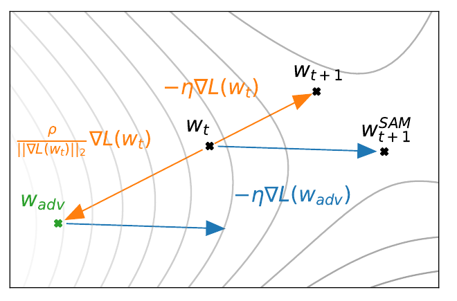
Let's walk through the figure. Starting at , ordinary SGD follows to at the upper right. SAM first goes the other way, a short distance uphill along the gradient, to , a first-order estimate of the highest-loss point within radius . Computing the gradient at gives the blue arrow ; move that arrow back so it starts at , and its tip is SAM's . The two endpoints lie in different directions; SAM moves in the direction that still goes downhill in the worst case.
So each step takes two forward and backward passes, twice the original compute. In PyTorch, with plain SGD as the base optimizer:
import torch

def sam_step(model, loss_fn, x, y, base_opt, rho=0.05):
    """One SAM update (p = 2): move to the worst point in the neighborhood, then use its gradient to update the original weights"""
    params = [p for p in model.parameters() if p.requires_grad]

    loss_fn(model(x), y).backward()                    # 1st backward pass: ∇L(w)
    with torch.no_grad():
        norm = torch.norm(torch.stack([p.grad.norm() for p in params]))
        eps = [rho * p.grad / (norm + 1e-12) for p in params]   # ε̂ = ρ ∇L / ‖∇L‖₂
        for p, e in zip(params, eps):
            p.add_(e)                                  # w → w + ε̂
    base_opt.zero_grad()

    loss_fn(model(x), y).backward()                    # 2nd backward pass: ∇L(w + ε̂)
    with torch.no_grad():
        for p, e in zip(params, eps):
            p.sub_(e)                                  # back to w
    base_opt.step()                                    # w ← w − η ∇L(w + ε̂)
    base_opt.zero_grad()
The norm here is computed over the gradients of all parameters concatenated into one vector, so the whole model shares a single .
How to choose
is the only hyperparameter SAM adds. The authors pick it from using 10% of the training data as a validation set, and the values chosen on CIFAR range from 0.02 to 0.2. They also call a “solid default”; the appendix reruns all the CIFAR and fine-tuning experiments with 0.05, and the results mostly match the tuned- versions or fall only slightly short, all still beating the baselines without SAM. Every ImageNet experiment uses 0.05.
Note that is an absolute distance in parameter space. The same 0.05 is a small perturbation for large weights and a large one for small weights. This will come up again later.
Discussion
Comparison conditions
Every experiment simply swaps SAM into the existing training procedure. Because SAM computes two gradients per step, the authors let the baselines without SAM run twice as many epochs and take the better of the standard and doubled lengths; they say the longer runs usually don't help noticeably. Each setting is run 5 times, reporting the mean and a 95% confidence interval. The implementation is in JAX; with multiple accelerators, each one computes and the SAM gradient on its own sub-batch, and the results are averaged at the end. This detail becomes very important later.
CIFAR
The CIFAR models are WideResNet, Shake-Shake and PyramidNet, all already well tuned and carrying plenty of regularization of their own. A few rows:
| Model and augmentation | CIFAR-10 | CIFAR-100 |
|---|---|---|
| WRN-28-10, 200 ep, basic | 2.7 / 3.5 | 16.5 / 18.8 |
| WRN-28-10, 1800 ep, AA | 1.6 / 2.2 | 12.8 / 16.1 |
| PyramidNet, basic | 2.7 / 4.0 | 14.6 / 19.7 |
| PyramidNet+ShakeDrop, AA | 1.4 / 1.6 | 10.3 / 10.6 |
Compiled from Table 1 of the paper; each cell is “SAM / SGD” test error (%), and AA is AutoAugment.
A plain WideResNet with SAM drops CIFAR-10 error from 2.2% to 1.6%, a level that used to take complex combinations like PyramidNet plus ShakeDrop. On the already heavily regularized PyramidNet+ShakeDrop, the improvement is much smaller, with CIFAR-100 going from 10.6% to 10.3%, but that was also the best result at the time without extra data.
ImageNet
ResNet-50, 101 and 152, batch size 4096, SGD with momentum, a cosine schedule, label smoothing, , and up to 400 epochs of training.
| Model | 100 ep | 200 ep | 400 ep |
|---|---|---|---|
| ResNet-50 | 22.5 / 22.9 | 21.4 / 22.3 | 20.9 / 22.3 |
| ResNet-101 | 20.2 / 21.2 | 19.4 / 20.9 | 19.0 / 22.3 |
| ResNet-152 | 19.2 / 20.4 | 18.5 / 20.3 | 18.4 / 20.9 |
Compiled from Table 2 of the paper; each cell is “SAM / standard training” top-1 error (%).
Read the table across. Standard training gets worse rather than better from 200 to 400 epochs, with ResNet-101 slipping from 20.9% to 22.3%, classic overfitting; SAM keeps improving. Matching compute instead, 200 epochs of SAM cost about as much as 400 epochs of standard training, and SAM still wins, 21.4% vs 22.3% for ResNet-50 and 18.5% vs 20.9% for ResNet-152. At 100 vs 200 epochs, though, ResNet-50 with SAM gets 22.5%, slightly behind standard training's 22.3%.
Fine-tuning
Fine-tuning starts from public EfficientNet checkpoints; EfficientNet-L2 had already been trained to 88.2% with NoisyStudent on ImageNet plus JFT. Fine-tuning with SAM lowers ImageNet top-1 error from 11.8% to 11.39%, CIFAR-100 from 4.07% to 3.92% and Stanford Cars from 4.93% to 4.04%; the ImageNet and CIFAR-100 results both set records at the time. BN statistics are frozen during fine-tuning, and ImageNet is trained for only 10 epochs.
Label noise
Since SAM looks for parameters whose whole neighborhood holds up under perturbation, the authors guessed it would also be more robust to noise in the training data. The experiment randomly scrambles part of the CIFAR-10 training labels, keeps the test set clean, and trains a ResNet-32 for 200 epochs:
| Method | 20% | 40% | 60% | 80% |
|---|---|---|---|---|
| SGD | 84.8 | 68.8 | 48.2 | 26.2 |
| Mixup | 93.0 | 90.0 | 83.8 | 70.2 |
| SAM | 95.1 | 93.4 | 90.5 | 77.9 |
| Bootstrap+SAM | 95.4 | 94.2 | 91.8 | 79.9 |
| MentorMix | 95.6 | 94.2 | 91.3 | 81.0 |
Compiled from Table 4 of the paper; the columns are noise rates and the values are accuracy (%) on the clean test set; the MentorMix numbers come from the literature.
With 80% of the labels wrong, SGD is down to 26.2% while SAM still gets 77.9%. SAM on its own beats every method built specifically for noisy labels except MentorMix; train once, then retrain with the model's own predictions as labels (Bootstrap), and it is about level with MentorMix. is 0.1 in these experiments, switched to 0.05 at 80% noise to converge stably.
m-sharpness: each device perturbs on its own
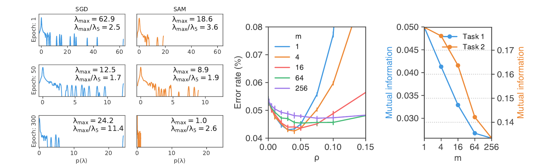
As mentioned earlier, with multiple devices each one computes its own perturbation. That amounts to changing the objective to “maximize separately over each group of examples, then sum,” where is the number of examples per device; the authors call this kind of sharpness m-sharpness.
Start with the middle plot. The vertical axis is labeled %, but the values are fractions, so 0.05 means 5%. At the error rate is about 5.3%. The minima for and are about 4.3%, but they degrade quickly once goes past 0.05; the purple line is the flattest, bottoming out only at about 4.7%. Small works better, which happens to suit multi-device parallelism. The right plot shows that the smaller is, the better m-sharpness predicts the actual generalization gap. From this, the authors argue that m-sharpness may describe generalization better than sharpness over the full training set.
The six small plots on the left confirm that SAM really does stop where curvature is lower. The model is a WideResNet-40-10 without BN, with the Hessian eigenvalue spectrum estimated by the Lanczos method; at the end of training, the largest eigenvalue is about 24 for SGD and about 1.0 for SAM, and , which describes the overall spread, drops from 11.4 to 2.6.
This section has a practical consequence. In PyTorch's DistributedDataParallel, backward() automatically averages the gradients across GPUs, so if the first backward pass syncs as usual, is computed from the whole batch and suddenly becomes large. davda54/sam recommends putting the first backward pass inside model.no_sync(), so that each GPU keeps its own perturbation.
Later understanding of SAM
Sharpness itself is shaky
Three years before SAM, Dinh et al. had already pointed out that the notion of “flatness” stands on shaky ground in deep networks. ReLU satisfies , so multiplying one layer's weights by and dividing the next layer's by leaves the function the network computes exactly the same, while stretching the shape of the loss landscape in parameter space. They proved it first for networks with a single hidden layer and then extended it to multiple layers, showing that for any minimum with a nonzero Hessian, you can find parameters with the same function and an arbitrarily large Hessian spectral norm. Same function means same generalization, yet the sharpness can be set at will, so sharpness measured in the raw parameter coordinates can't by itself explain generalization.
SAM's has the same problem, since it is an absolute distance in parameter space. ASAM (Kwon et al., 2021) scales the perturbation range by weight magnitude, changing the constraint to with , and this “adaptive sharpness” is invariant under the rescaling above. With , the perturbation becomes , so coordinates with larger weights get larger perturbations, and has to be about 10 times larger as a result (0.5 for CIFAR-10, 1.0 for CIFAR-100). ResNet-50 top-1 accuracy on ImageNet is 75.79%, 76.39% and 76.63% for SGD, SAM and ASAM, respectively.
Generalization bounds can't explain SAM
Andriushchenko and Flammarion (2022) went back to check SAM's theoretical basis. The generalization bound leads to a version that maximizes over the full training set, which they call n-SAM; what the paper actually uses is m-SAM, which perturbs per batch. Measured on CIFAR, random perturbations barely help, n-SAM barely helps either, and only low- versions (such as 128-SAM) clearly improve generalization. If the bound were the reason, n-SAM should be best; the results show the exact opposite. They conclude that existing generalization bounds can't explain SAM, and that being “flatter” as measured by m-sharpness doesn't necessarily bring better generalization.
They also offer some usable observations. On diagonal linear networks, 1-SAM's implicit bias favors sparser solutions, more strongly than n-SAM or ordinary training; on CIFAR, switching from ordinary training to SAM for only the last 10% or so of epochs clearly improves generalization, so SAM can be used to fine-tune existing models.
In 2023, Andriushchenko et al. widened the scope to Transformers on ImageNet, CLIP fine-tuning and BERT. Sharpness (including adaptive sharpness) correlated poorly with generalization and correlated instead with training settings such as the learning rate; in several cases, sharper minima did better on out-of-distribution data.
Widely used
Whatever the theorists are arguing about, SAM is widely used in practice. Chen et al. (2022) found that ViTs trained from scratch on ImageNet, without large-scale pretraining and with only simple data augmentation, converge to extremely sharp minima; with SAM, ViT-B/16's top-1 rises from 74.6% to 79.9%, and MLP-Mixer-B/16's from 66.4% to 77.4%. NFNet's largest model, F6, also needed SAM to reach its 86.5% accuracy.
Conclusion
SAM turns “the loss should be low across the whole neighborhood” into a min-max objective, uses a first-order approximation to turn the inner maximization into “walk uphill along the gradient,” and then takes the gradient at that point to update the original weights. The cost is two backward passes per step. It wins broadly on CIFAR, ImageNet, fine-tuning and noisy labels, and in the CIFAR comparisons the baselines even got twice the epochs.
In practice, is a good starting point, and plan for twice the compute. With BN models, remember not to update the statistics on the second forward pass; with multiple GPUs, don't sync the first backward pass, so each GPU perturbs on its own. If compute is short, you can switch SAM on only for the last stretch of training, or only for fine-tuning.
As for “flat means it generalizes,” papers were still arguing against it in 2023; SAM, meanwhile, has kept getting used.