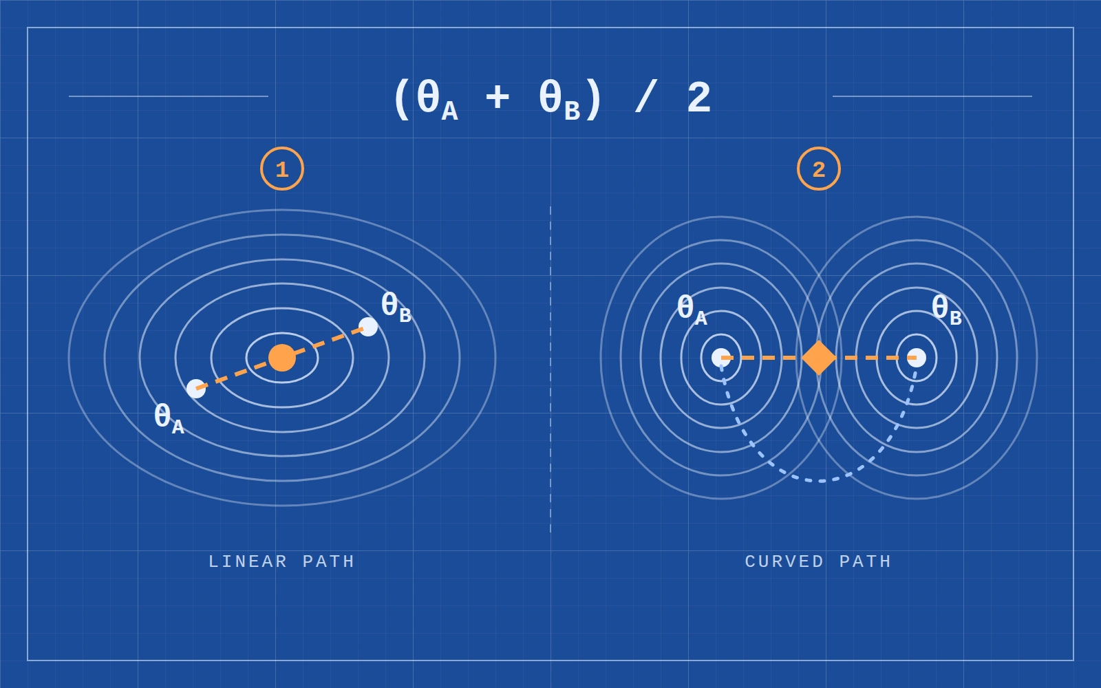
In February 2016, Brendan McMahan and colleagues at Google posted a paper on arXiv introducing the federated learning algorithm later known as FedAvg. Each device trains a model on its own data; the server averages the weights it receives.
There is an obvious concern. A neural network's loss function is nonconvex. As the authors themselves point out, averaging two models in parameter space can produce an arbitrarily bad result.
They began with a small experiment. Two MNIST classifiers, each with two hidden layers, were trained for 240 steps on separate, nonoverlapping sets of 600 handwritten digits. They then interpolated between the two sets of weights and measured the resulting model's loss on the full training set.
When the two models used different random seeds for their initial weights, the loss shot up halfway between them. With the same seed, the averaged model had lower loss than either parent. FedAvg Figure 1
Look at the curves the authors actually measured. The horizontal axis is the weight mixing coefficient; the vertical axis is loss on the full MNIST training set. The two panels use different vertical scales. The left curve rises into a hill in the middle, while the right curve dips below both endpoints.
This observation occupies just one small figure in the paper's second section.
Eight years later, merged models crowded the top of Hugging Face's Open LLM Leaderboard. Community tutorials described merging as a cheap way to create models, with “no GPU required.” By March 2024, the leaderboard team had hidden merged models by default.
A year later, Cohere used weighted averaging to combine six experts into the 111-billion-parameter Command A, losing just 1.8% on average relative to the individual experts. In April 2026, DeepSeek-V4 also trained a collection of experts, but chose distillation to transfer their abilities into one model. Its technical report explicitly says this avoids the performance degradation often associated with weight merging.
We will start from that small figure. First, we will average two models on a laptop, see how it fails, and fix it. Then we will follow the story forward: how “add and divide by two” went from a small federated learning experiment to leaderboard alchemy, and then into model developers' training pipelines.
The first half covers the mechanism: why different starting points can resist averaging, and how alignment and a shared starting point address the problem.
The second half covers applications, from soups of fine-tuned models and task vectors to leaderboards and training pipelines.
First, average two models on a laptop
We will follow the FedAvg setup, replacing MNIST with scikit-learn's built-in digits dataset: 1,797 handwritten 8×8 digits, with no separate download. The architecture, learning rate, batch size and step count follow the paper: two hidden layers of 200 units each, learning rate 0.1, batch size 50, and 240 training steps.
import torch
import torch.nn as nn
from sklearn.datasets import load_digits

X, y = load_digits(return_X_y=True)                    # 1,797 張 8×8 的手寫數字
X = torch.tensor(X / 16.0, dtype=torch.float32)
y = torch.tensor(y)
perm = torch.randperm(len(X), generator=torch.Generator().manual_seed(0))
idx_a, idx_b, idx_test = perm[:600], perm[600:1200], perm[1200:]

def make(seed):
    torch.manual_seed(seed)                            # 種子決定初始權重
    return nn.Sequential(nn.Linear(64, 200), nn.ReLU(),
                         nn.Linear(200, 200), nn.ReLU(),
                         nn.Linear(200, 10))

def train(model, idx, seed):
    opt = torch.optim.SGD(model.parameters(), lr=0.1)
    g = torch.Generator().manual_seed(seed)            # 種子決定資料順序
    for epoch in range(20):                            # 600 張、批次 50,共 240 步
        order = idx[torch.randperm(len(idx), generator=g)]
        for b in order.split(50):
            loss = nn.functional.cross_entropy(model(X[b]), y[b])
            opt.zero_grad()
            loss.backward()
            opt.step()
    return model
make sets the initial-weight seed; train sets the data-order seed. The two training sets contain 600 images each, with no overlap. The remaining 597 images form the test set.
Next, we need two small helpers. mix mixes the two sets of weights using coefficient :
gives their arithmetic mean. evaluate reports loss on the combined training sets and accuracy on the test set.
def mix(m1, m2, t):
    sd1, sd2 = m1.state_dict(), m2.state_dict()
    merged = make(0)
    merged.load_state_dict({k: t * sd1[k] + (1 - t) * sd2[k] for k in sd1})
    return merged

@torch.no_grad()
def evaluate(model):
    seen = torch.cat([idx_a, idx_b])                   # 兩份訓練資料合起來
    loss = nn.functional.cross_entropy(model(X[seen]), y[seen]).item()
    acc = (model(X[idx_test]).argmax(1) == y[idx_test]).float().mean().item()
    return f"loss {loss:.3f}, 測試 {acc:.1%}"

for name, seed_a, seed_b in [("不同起點", 1, 2), ("同一起點", 1, 1)]:
    A = train(make(seed_a), idx_a, seed=10)
    B = train(make(seed_b), idx_b, seed=20)
    print(name)
    print("  A   :", evaluate(A))
    print("  B   :", evaluate(B))
    print("  平均:", evaluate(mix(A, B, 0.5)))
不同起點
  A   : loss 0.264, 測試 92.1%
  B   : loss 0.270, 測試 93.0%
  平均: loss 1.277, 測試 83.4%
同一起點
  A   : loss 0.264, 測試 92.1%
  B   : loss 0.266, 測試 93.3%
  平均: loss 0.252, 測試 93.6%
The models trained from different starting points achieve about 92% and 93% test accuracy individually. Averaging drops accuracy to 83.4% and raises loss from around 0.27 to 1.277.
For the shared-start pair, the averaged model's loss is 0.252, below A's 0.264 and B's 0.266. Test accuracy reaches 93.6%, also above both parents. Each model has seen only half the training data, yet their average performs better on the combined training set than either parent. This small dataset reproduces the trend in the right-hand panel of FedAvg's figure.
Here we train separately once and average once. Full FedAvg sends the averaged model back to the devices, lets each update it for a few steps, and averages the returned weights in proportion to local dataset sizes, repeatedly. Our datasets are equal in size, so adding and dividing by two is enough. Unequal dataset sizes require unequal coefficients. Understanding this one round makes the multi-round procedure easier to follow.
Sweep from 0 to 1 to see the whole curve:
Repeating the experiment with five seed pairs gives the same pattern. Averaged across the five runs, parent-model test accuracy is 92.9%; directly averaging different starts gives 80.2%; averaging a shared-start pair gives 93.6%. The last decimal places can vary across machines or PyTorch versions.
The same network in a different order
Why can different starting points resist averaging? Consider an even more extreme example.
The 200 hidden units have no fixed order. Swap units 3 and 7, and swap the corresponding input positions in the next layer: the network computes exactly the same function. Rows of its weight matrix have changed places; its function has stayed the same.
Hecht-Nielsen discussed this permutation symmetry in 1990. Git Re-Basin §1
Our network has two hidden layers of 200 units each. Permutation alone gives equivalent parameterizations, roughly . Every one represents the same model.
Now average model A with “A in a shuffled order”:
def permute(model, p1, p2):
    sd = {k: v.clone() for k, v in model.state_dict().items()}
    sd["0.weight"], sd["0.bias"] = sd["0.weight"][p1], sd["0.bias"][p1]  # 第一層的 200 個單元換位
    sd["2.weight"] = sd["2.weight"][:, p1]                              # 下一層讀輸入的順序跟著換
    sd["2.weight"], sd["2.bias"] = sd["2.weight"][p2], sd["2.bias"][p2]  # 第二層的 200 個單元換位
    sd["4.weight"] = sd["4.weight"][:, p2]
    out = make(0)
    out.load_state_dict(sd)
    return out

A = train(make(1), idx_a, seed=10)
g = torch.Generator().manual_seed(100)
A2 = permute(A, torch.randperm(200, generator=g), torch.randperm(200, generator=g))

print(torch.allclose(A(X), A2(X), atol=1e-5))         # 每一張圖的輸出都一樣嗎?
print("A   :", evaluate(A))
print("A2  :", evaluate(A2))
print("平均:", evaluate(mix(A, A2, 0.5)))
True
A   : loss 0.264, 測試 92.1%
A2  : loss 0.264, 測試 92.1%
平均: loss 1.215, 測試 84.3%
True means that their outputs on all 1,797 images agree to within one part in 100,000. Both achieve 92.1% accuracy. Yet averaging them drops accuracy to 84.3%.
Even averaging a model with itself can fail when the units are misaligned. Averaging works by position: unit 3 in A is averaged with whatever occupies slot 3 in A2. That slot actually holds a different unit from A, detecting a different feature. Half of each of two unrelated detectors often produces something unlike either one.
Independently seeded models can have a similar problem. They may have learned similar features in different positions.
Align first, then average
If order is the problem, align the order first. In 2021, Entezari et al. proposed a bold conjecture: once all possible permutations are taken into account, SGD solutions generally have no barrier along the straight segment between them. Entezari et al.
Git Re-Basin, published in 2022, provides ways to find those permutations. Its simplest method, weight matching, needs no data. For each layer, compute the similarity between every pair of units in A and B, then solve a linear assignment problem—classically with the Hungarian algorithm—to find the one-to-one matching with the highest total similarity. Similarity includes a unit's incoming weights, bias and outgoing weights. Since the two layers' permutations affect one another, repeat the process for several passes.
from scipy.optimize import linear_sum_assignment

def match(ref, other, iters=20):
    a, b = ref.state_dict(), other.state_dict()
    p1, p2 = torch.arange(200), torch.arange(200)
    for _ in range(iters):
        # 第一層:比對每個單元的輸入權重、偏差,以及它送往下一層的權重
        s1 = (a["0.weight"] @ b["0.weight"].T
              + torch.outer(a["0.bias"], b["0.bias"])
              + a["2.weight"].T @ b["2.weight"][p2])
        p1 = torch.as_tensor(linear_sum_assignment(s1.numpy(), maximize=True)[1])
        # 第二層:同樣的比對,輸入端改用剛排好的 p1
        s2 = (a["2.weight"] @ b["2.weight"][:, p1].T
              + torch.outer(a["2.bias"], b["2.bias"])
              + a["4.weight"].T @ b["4.weight"])
        p2 = torch.as_tensor(linear_sum_assignment(s2.numpy(), maximize=True)[1])
    return permute(other, p1, p2)

A = train(make(1), idx_a, seed=10)
B = train(make(2), idx_b, seed=20)
B2 = match(A, B)
print(torch.allclose(B(X), B2(X), atol=1e-5))         # 換位不改變 B 的功能
print("直接平均  :", evaluate(mix(A, B, 0.5)))
print("對齊後平均:", evaluate(mix(A, B2, 0.5)))
True
直接平均  : loss 1.277, 測試 83.4%
對齊後平均: loss 0.383, 測試 91.6%
After permutation, B2 produces exactly the same outputs as B. Averaging it with A restores test accuracy from 83.4% to 91.6% and lowers loss from 1.277 to 0.383. This is the light-blue curve above: the central hill is much lower.
Across five seed pairs, accuracy recovers from 80.2% to 92.2%. Alignment recovers most of the loss, but still trails the shared-start pair's 93.6%; its loss also remains above both parents.
Git Re-Basin finds a similar pattern in larger models. On CIFAR-10, two independently trained ResNet-20 models widened by 32× reach zero barrier after alignment—the first such result known to the authors. Standard-width ResNet-50 on ImageNet sees a 67% reduction, with some barrier remaining. Wider networks are more likely to become connected after alignment. Git Re-Basin
These interpolation curves show both the success and its limits. Gray is direct interpolation; green is weight matching. The widened ResNet-20 in the third panel is almost flat, while the standard-width ResNet-50 at the right retains a hump. Solid lines measure training loss and dashed lines test loss; read both.
The CIFAR experiments also replace normalization with LayerNorm. ImageNet retains BatchNorm and reestimates its statistics after interpolation. Alignment must handle biases, normalization and residual branches together; sorting each layer's rows alone leaves work unfinished. Our earlier MLP omits those components, which makes a few dozen lines of code sufficient.
This route works, but it requires an assignment problem at every layer and a sufficiently wide network.
Start from the same place
Another route avoids the permutation search by giving the models a shared training history.
FedAvg uses identical initial weights. In 2019, Frankle et al. studied this systematically. They duplicated a network, continued training with different data orders and augmentations, and checked the straight-line barrier between the resulting models. Only the smallest MNIST network had no barrier from initialization. Other networks needed a short shared training phase first: about 3% of training for ResNet-20 on CIFAR-10, and 20% for ResNet-50 on ImageNet. After that point, the sampled training runs ended in linearly connected regions. Frankle et al., §1
Their stability criterion is a maximum interpolation error less than two percentage points above the average endpoint error. When ResNet-20 first meets it, test error is still around 25%, versus 8.3% at the end of training. Learning is far from complete; the eventual endpoints have simply become easier to interpolate. Shared initialization and a shared trained trajectory therefore need to be considered separately.
Move the duplication point later in training and you get these five plots. Instability is on the vertical axis; red measures test data and purple training data. MNIST LeNet stays near zero from the start, while the others need some shared training. The first three plots use iterations and the last two epochs, so check the time units too.
Our little MLP appears to fall into the smallest-network category: sharing the initialization seed was enough in the experiment above.
Different basins can also be connected. In 2018, Garipov et al. and Draxler et al. independently found curved paths of nearly constant loss between independently trained solutions. The straight segment still hits a high wall; the curved dashed path in the right-hand schematic illustrates the detour. Garipov et al., Draxler et al.
In the original figure, the colors encode measured loss. Straight segments between the three independent solutions on the left cross high-loss regions. The Bézier curve in the middle and polygonal chain on the right connect the endpoints through low-loss regions. Training has supplied a path; the arithmetic midpoint of the endpoints has stayed in place.
That same year, Izmailov, a coauthor of Garipov's paper, and colleagues proposed SWA. They average checkpoints from a single training run. A relatively high constant or cyclical learning rate keeps SGD moving around the basin, and their weights are averaged equally. The paper traces trajectory averaging back to Ruppert's 1988 work. On ImageNet, another 10 SWA epochs from a trained ResNet-50 raise top-1 accuracy from 76.15% to 76.97%. The authors argue that the average lies in a flatter region and generalizes better. SWA Table 2
These CIFAR-100/ResNet-164 slices make that explanation concrete. The three crosses in the left panel are FGE samples, with their mean between them. The middle panel shows test error; the right shows training loss. SGD and SWA have different relative performance in the two panels: the lowest training loss can occur away from the lowest test error.
These three ideas serve different purposes. Mode connectivity establishes that a curved low-loss path can be trained. Linear mode connectivity requires the straight segment to work too, which directly concerns weight averaging. SWA collects nearby checkpoints along one trajectory and produces a single deployment model. When only a curved channel connects the endpoints, their average can still fall outside it.
SWA also gives a local explanation for why averaging can resemble ensembling. Let the checkpoint mean be and each deviation be , so . Expand the network output around the mean:
The first-order terms cancel. The difference between output ensembling and the averaged-weight model is second order. This explains how nearby checkpoints can let one model approximate an ensemble. When the points are far apart or local nonlinearity is strong, those second-order terms matter. BatchNorm statistics must also be reestimated for the averaged model. Check proximity and low loss along the segment before applying the argument.
Pretrained models made a shared starting point widely available. In 2020, Neyshabur et al. observed that models fine-tuned from the same pretrained weights stay in the same basin, learn similar features and remain close in parameter space. Models trained from random initialization lack this property. Neyshabur et al.
When everyone starts from the same CLIP or Llama, fine-tuned models are siblings with a shared starting point. From here, fine-tuning becomes the main arena for model merging.
A pot of soup
The usual training workflow runs several hyperparameter settings, keeps the model with the best validation score and discards the rest.
WiSE-FT offered a simple alternative in 2021. Zero-shot CLIP is fairly robust to distribution shifts. Fine-tuning improves ImageNet accuracy but hurts shifted distributions. WiSE-FT linearly mixes the zero-shot and fine-tuned weights. Across five ImageNet-derived shift datasets, it improves over previous approaches by four to six percentage points, while adding 1.6 points on ImageNet itself, at the same inference cost. WiSE-FT
The coefficient curves show all six datasets. On the horizontal axis, is the zero-shot model and the fine-tuned model. Pink traces the interpolated models; the horizontal dotted line marks the better endpoint. Several datasets peak in the middle, but at different locations. A single coefficient cannot automatically optimize every distribution.
In 2022, Model Soups turned to the models that would otherwise be discarded. The authors fine-tuned CLIP ViT-B/32 on ImageNet 72 times, using randomly sampled hyperparameters:
- Best individual model: 80.38%
- Average all 72 models (uniform soup): 79.97%, worse than the best individual model
- Greedy soup: 81.03%
- Output ensemble of all 72 models: 81.19%, but requiring 72 model evaluations at inference
These numbers come from the ImageNet column of the original table. The Dist. shifts column on the right averages five shifted datasets; uniform soup beats greedy soup there. The validation data used to select members affects which tests the final model handles best.
Greedy soup uses a simple recipe. Sort models by validation accuracy, start with the best, and try adding the others one at a time. Keep a candidate if validation performance does not decrease; skip it otherwise. Some hyperparameters, such as an excessive learning rate, can send a model into another basin. Uniform averaging suffers from those models; greedy soup leaves them out.
This CLIP soup ends up with five members. If the soup already contains models, the next candidate is . Repeatedly averaging half and half would give later arrivals more weight. Members are selected using roughly 2% of the ImageNet training set held out for this purpose; the official validation set remains the test set. Each trial evaluates a new candidate model, although it needs no further backpropagation.
Greedy soup guarantees no regression on the selection data; test performance must be measured separately. Output ensembles also improve probability calibration, a benefit the soups fail to match in the paper's calibration experiments. Soup is attractive when a single model and classification accuracy are the priority. If probabilities determine abstention or human review, compare calibration too.
For ViT-G/14 pretrained on JFT-3B, greedy soup selects 14 of 58 fine-tuned models and reaches 90.94% on ImageNet. It surpasses the then-best CoAtNet-7's 90.88%, with 25% less inference computation. Model Soups Table 1, Table 3
Every model in this pot handles the same task. Next, we will put models for different tasks into one pot.
Task vectors
In late 2022, Ilharco et al. described fine-tuning as a direction. Let the pretrained weights be and the weights fine-tuned on task A be . Subtract them:
is a task vector: it records the direction and size of every weight change made for task A. Now we can do arithmetic:
Adding several task vectors attempts to give one model all their tasks. Negating a vector and adding it tests whether the corresponding behavior can be reduced while retaining others. The coefficient is selected using held-out validation data.
The paper experiments with CLIP on eight image-classification datasets, covering car models, textures, satellite imagery and house numbers. Adding two task vectors retains 98.9% of the experts' accuracy on those two tasks on average. With all eight vectors available, the best multitask model reaches 91.2%. Multitask fine-tuning on all eight datasets reaches 99.4%. Merging avoids retraining and access to the original datasets, while leaving a performance gap. Task Arithmetic, §4 and Appendix D
In this ViT-L/14 plot, accuracy on each of the eight tasks is divided by that task's specialist accuracy and then averaged. Pale dots represent different subsets of task vectors; the dark line averages subsets of the same size. Adding more vectors improves overall ability, with a remaining gap to 1.0, where every task would match its specialist.
Subtraction works too. Subtracting GPT-2 Large's task vector from fine-tuning on toxic comments lowers the fraction classified as toxic from 4.8% to 0.8% among 1,000 generations under fixed prompts. WikiText-103 perplexity changes from 16.4 to 16.9. This changes behavior under a specific evaluation; verifying removal of a particular piece of information requires a separate protocol. Task Arithmetic §3
Why does addition work? In 2023, Ortiz-Jimenez et al. argued that weight disentanglement is key: different task vectors affect disjoint regions of the input space, limiting interference when added. Repeating the experiment with a randomly initialized ViT produces multitask accuracy near chance. This comparison supports the role of pretraining in providing a structure for task disentanglement. Ortiz-Jimenez et al., §6.2
Task arithmetic therefore shares the premise of the FedAvg figure: the models need a common starting point, preferably a pretrained one.
A shared start provides common coordinates, but task vectors still overlap at individual parameters. The original paper reports cosine similarities of just 0.01–0.03 for most CLIP task-vector pairs, rising to about 0.18 for related tasks such as MNIST and SVHN. Near-orthogonality helps explain limited interference, but the effect of each change on actual outputs still matters. TIES, introduced next, addresses local parameter conflicts even when the full task vectors are nearly orthogonal.
When parameters clash
The earlier 91.2% measures retention relative to specialists. Now consider the smaller CLIP ViT-B/32 setup in TIES-Merging. Its eight separately fine-tuned specialists average 90.5% accuracy. Task arithmetic combines them into one model scoring just 70.1%, even with a validation-selected coefficient. These raw accuracies show how difficult retaining all eight abilities remains. TIES-Merging Table 1
Read down the ViT-B/32 column in the original table. The specialists score 90.5, task arithmetic with validation scores 70.1, and TIES reaches 73.6. The upper and lower halves differ in their Validation column. The 70.1 result and the upper half's 60.4 use different coefficient-selection conditions and belong to separate comparisons.
Yadav et al. attribute the degradation to two kinds of interference. First is redundancy: many fine-tuned parameters move only slightly and contribute little to a task, yet dilute larger, useful changes from others when averaged. Second is sign conflict: task A wants a parameter to increase while task B wants it to decrease, so addition cancels the changes. Conflicts already occur with two models and affect more parameters as more models are merged. TIES-Merging §3
Work through three tasks and six parameters using numbers chosen for illustration:
import numpy as np

tau = np.array([[ 0.8, -0.1,  0.5,   0.02, -0.6, 0.3 ],   # 任務 A
                [-0.7,  0.4,  0.6,  -0.03,  0.1, 0.05],   # 任務 B
                [ 0.9, -0.2, -0.05,  0.01, -0.5, 0.4 ]])  # 任務 C

print("直接平均:", tau.mean(0).round(3))

# 1. Trim:每個任務只留絕對值最大的一半
k = tau.shape[1] // 2
cut = np.sort(np.abs(tau), axis=1)[:, -k][:, None]
trimmed = np.where(np.abs(tau) >= cut, tau, 0.0)
print(trimmed)

# 2. Elect:每個參數用剩下數值的總和投票,決定正負號
sign = np.sign(trimmed.sum(0))

# 3. Merge:只平均和投票結果同號的值
agree = (np.sign(trimmed) == sign) & (trimmed != 0)
ties = (trimmed * agree).sum(0) / np.maximum(agree.sum(0), 1)
print("TIES    :", ties.round(3))
直接平均: [ 0.333  0.033  0.35   0.    -0.333  0.25 ]
[[ 0.8  0.   0.5  0.  -0.6  0. ]
 [-0.7  0.4  0.6  0.   0.   0. ]
 [ 0.9  0.   0.   0.  -0.5  0.4]]
TIES    : [ 0.85  0.4   0.55  0.   -0.55  0.4 ]
Start with parameter 0. A and C want it larger (+0.8 and +0.9); B wants it smaller (−0.7). Direct averaging leaves 0.333. TIES elects a sign from their sum, which is positive, and averages only A and C to obtain 0.85.
Parameter 1 illustrates redundancy. Only B makes a substantial change (+0.4); A and C move by −0.1 and −0.2. Averaging cancels much of B's change, leaving 0.033. Trimming the small values preserves B's 0.4. At parameter 3, every change is just a few hundredths, so trimming sets the whole coordinate to zero.
The name comes from these steps: Trim, Elect sign, and Merge values with the elected sign. The paper retains the largest 20% of each task vector by magnitude, after checking that keeping this fraction preserves roughly the same individual-task performance as the full vector. The merged vector is scaled by and added back to the pretrained weights.
Step 2 uses the sum of signed values rather than a head count: against two values still elects positive. The final divisor is the number of retained, nonzero members with that coordinate's elected sign; trimmed zeros are excluded. The evidence for keeping just 20% comes from parameter-efficient fine-tuning of T0-3B, before testing the recipe with fully fine-tuned T5 and CLIP. Sweep the retention fraction for your own tasks.
On ViT-B/32's eight tasks, TIES reaches 73.6% with validation data, versus task arithmetic's 70.1%. Without validation it reaches 72.4%, versus 60.4%. Both remain far below the separately fine-tuned specialists' 90.5%.
The authors also test an oracle: take signs from an already trained multitask model instead of electing them from summed task vectors. Across eleven parameter-efficient fine-tuning tasks, this gives 72.0%, close to the multitask model's 73.1%, versus standard TIES at 66.4%. Better directions offer substantial headroom, but the oracle has already required full multitask training.
Drop ninety percent
DARE, introduced in November 2023, goes further. For each fine-tuned model, it randomly drops a fraction of the difference from the pretrained model—the delta parameters—and scales the rest by .
Why rescale? Each value survives with probability and is multiplied by when retained, so its expected value equals the original:
The drop fraction can be huge. The authors observe that most deltas after supervised fine-tuning of language models are within 0.002. Redundancy is high enough that dropping 90%, or even 99%, often has little effect. Larger models tolerate larger ; at 70 billion parameters, dropping 99% has little effect in their experiments. DARE performs the dropping; task arithmetic or TIES then performs the merge. DARE §1
The left panel makes the scale difference clear. Drop rate is on the horizontal axis and GSM8K accuracy on the vertical. At 0.99, the 7B model drops sharply while 70B stays near its original score. The right panel shows three post-merge evaluations; language, math and coding retention need separate measurements.
The paper is equally clear about failure with large deltas. Continued pretraining can produce deltas around 0.03, where DARE fails. WizardCoder-Python-13B is fine-tuned from CodeLlama-13b-Python: its deltas relative to that base stay within 0.0002, but often exceed 0.01 relative to Llama 2. Dropping relative to Llama 2 causes problems.
That failure is dramatic: dropping just 10% reduces HumanEval and MBPP pass@1 from 63.41 and 55.4 to zero. The expectation identity still holds, but the variance of a single sample is . Large deltas, combined with high drop rates that amplify the few survivors, make outputs hard to preserve. The observed 0.002 scale must be interpreted alongside layerwise values and data distributions; it is unsuitable as a universal cutoff.
As a merge preprocessing step, DARE has mixed results. Task arithmetic on two 13B instruction and math experts scores 66.34% on GSM8K; adding DARE gives 66.26%. With TIES, DARE instead raises 15.77% to 36.16%. For task arithmetic combining three experts, GSM8K falls from 58.45% to 56.48%. TIES addresses direction conflicts and averaging interference; DARE reduces overlapping deltas. They act at different stages, and their combination still needs evaluation.
One detail is easy to miss. DARE drops deltas while retaining the complete base weights. The reconstructed model is still a dense model of the same size. Keeping 1% of the changes leaves inference computation essentially intact. DARE helps merging and delta sparsification; deployment acceleration requires additional work.
The DARE paper also uses the method to merge a 7B model that tops the Open LLM Leaderboard's 7B category, using only CPUs for the merge.
Around the same time, the community was already experimenting enthusiastically.
Alchemy without a GPU
On November 5, 2023, Goliath-120B appeared on Hugging Face. Its author took layer ranges from two fine-tuned Llama 2 70B models, Xwin and Euryale, and interleaved them into a deeper model, without further gradient training during the merge. Goliath-120B model card The community calls this a frankenmerge, after Frankenstein: parts of different models assembled into a new one. Strictly speaking, it averages no weights at all.
Charles Goddard's mergekit provides the assembly tools. Linear averaging, SLERP, task arithmetic, TIES, DARE and direct layer stacking through passthrough can all be specified in a configuration file. CPU merging is possible when memory is limited. Its March 2024 paper reports enabling thousands of merged models. Upstage's SOLAR-10.7B also starts with this kind of stacking, followed by continued pretraining. MergeKit
“No GPU required” refers to reading source tensors, combining them and writing a new checkpoint. The source models' training has already incurred its compute cost. Evaluation and inference still require running the resulting model. Goliath's deeper stack also increases its inference path and weight storage. It avoids extra gradient training while retaining the deployment requirements of a 120B-class model.
“Merging” therefore covers several operations. Weight interpolation at fixed depth preserves the architecture. Passthrough changes the number of connected layers. SOLAR adds a learning phase after stacking. Cost comparisons need to separate model creation, evaluation and deployment.
Why follow an arc?
SLERP stands for spherical linear interpolation. Ken Shoemake introduced it in a 1985 computer-animation paper to interpolate smoothly between rotations. In early 2024, it became the community's most popular merging method, although it merges only two models at a time.
Two vectors illustrate the issue. For perpendicular unit vectors and , direct averaging gives with length . SLERP follows the circular arc, giving midpoint with length 1:
The community's explanation is that linear interpolation in high dimensions shortens the weight vector, while changes in direction often matter more than changes in length. Labonne, 2024-01-09 The comparison above uses equal-length unit vectors. Real models require measuring each layer's norms and angles. If two fine-tuned models make small changes relative to a shared base and have a small mutual angle, , the two coefficients approach and , bringing SLERP close to linear interpolation. This is the formula's small-angle approximation. A delta magnitude reported by DARE alone cannot establish the angle between full models. Later, we will see that Cohere tried SLERP on its 111-billion-parameter model without finding a clear benefit.
The leaderboard
On January 9, 2024, Maxime Labonne published a mergekit tutorial on the Hugging Face blog. It opens by describing merging as a cheap way to create models without a GPU, responsible for many leading Open LLM Leaderboard entries. His SLERP merge, Marcoro14-7B-slerp, became the best 7B entry in early January. The same article openly acknowledges that merging leading models also combines their contamination, and advises assuming that Marcoro14-7B-slerp is contaminated. Labonne, 2024-01-09
Contamination means evaluation questions entering training data. Leaderboard questions are public and can be used to train models. Merges are especially hard to trace: a model's parents may themselves be merges, with fine-tuning at each generation.
In March 2024, Sakana AI introduced evolutionary model merging. The paper opens by observing that merged models dominate the Open LLM Leaderboard, and that merging is often treated as intuition-driven black magic or alchemy. Their solution uses an evolutionary algorithm to search both merging recipes and dataflow through layers from different models. Their Japanese math model, EvoLLM-JP, has only 7B parameters, scores 52.0 on MGSM-JA, and beats several earlier Japanese 70B models on multiple Japanese benchmarks. Akiba et al.
Later versions explain the setup more fully. Three Japanese and math models from the Mistral-7B family supply the weights. The main parameter-space search varies only density and weight per source, avoiding unnecessary layerwise degrees of freedom. Search uses 1,069 separately translated questions, leaving the final 250 MGSM-JA questions untouched. Parameter-space merging reaches 52.0%; adding dataflow search reaches 55.2%, with the model growing from 7B to 10B. Selecting the recipe on separate data allows transfer to be evaluated. Akiba et al., §3.1
The original figure distinguishes the operations through layer colors. Parameter-space search mixes source tensors into new ones; dataflow-space search selects source layers and their traversal order. Combining them changes both tensor values and dataflow. The three searches can produce different model sizes and forward paths.
By then, the leaderboard was hiding merges by default. On March 11, a merged-model author opened a discussion to protest: their model had repeatedly ranked first, yet the merge label hid it alongside flagged and deleted models, effectively stigmatizing it.
Hugging Face's Clémentine Fourrier explained that the fundamental problem was nearly untraceable ancestry. Fine-tuning Llama gives a known base and fine-tuning dataset. Merges can involve multiple generations of merges and deleted models, making data provenance hard to establish and accidental contamination easy. After repeated merging, fine-tuning and DPO, academic benchmark scores often fail to translate into useful performance. This was the reason for hiding them by default. Open LLM Leaderboard discussion #629
The dispute concerns both source transparency and evaluation selection. Repeatedly using a benchmark to choose parents or coefficients makes that benchmark part of the recipe search. Whether its test questions also entered training requires separate provenance checks. Keep a final test outside recipe selection, then examine outputs for the intended use. The discussion presents contamination concerns and moderation reasons; it provides no individual contamination finding for every merged model.
Entering the training pipeline
Beyond leaderboards, merging became common inside model developers' own training pipelines.
Public technical reports most often describe averaging several runs of a shared recipe:
- Llama 3 (July 2024): reward-model, SFT and DPO stages each average models trained with different data versions or hyperparameters. Llama 3 §4.1.5 For vision SFT, a hyperparameter sweep is ranked by performance and the top K models are averaged. The authors report consistent gains over the best individual grid-search model and lower hyperparameter sensitivity. Llama 3 §7.5.2
- Gemma 2 (July 2024): averages post-training runs with different hyperparameters, citing Google DeepMind's WARP. Gemma 2 §4
- OLMo 2 (December 2024): for 7B mid-training, processes the same 50B tokens in three different orders, then averages. Across six data mixtures, the average matches or beats the best individual run. OLMo 2 Table 14
- Tülu 3 (November 2024): tests soups of SFT runs with different seeds. The best soup and best individual seed perform similarly, so the authors consistently use the best individual run. Tülu 3 Table 14
The Tülu 3 result deserves attention: averaging sometimes brings no improvement.
Pretraining uses it too. ByteDance Seed's PMA averages checkpoints under a constant learning rate, testing models from a 411-million-parameter dense network to a 200-billion-parameter MoE. The averages improve performance and help predict performance after learning-rate annealing. Ant Group's WSM goes further, replacing the learning-rate decay phase with checkpoint merging. PMA, WSM
The objects being averaged differ. SWA and constant-learning-rate checkpoint averaging collect times along one trajectory. Model Soups and different-data-order experiments branch from a common checkpoint and train separately. The former require choosing a sampling start and duration; the latter require selecting branches for the soup. Both depend on compatible parameter coordinates and reevaluation after averaging.
Six experts, two soups
Cohere's April 2025 Command A technical report places merging at the center of the workflow.
The 111-billion-parameter Command A first trains a general instruction model, then branches into six experts for code, safety, RAG, math, multilingual and general long-context abilities. These SFT experts merge into an “SFT soup.” Domain-specific preference optimization and reinforcement learning from that soup produce the six experts the report calls RL experts. They are merged once more, followed by polishing. Command A §3
Merging uses simple linear weighted averaging, with coefficients chosen by heuristics and brute-force search. The report says more elaborate methods, including SLERP and task vectors, increased complexity without clear gains. Linear merging also has an engineering advantage: a merge of merges can be expressed as one linear merge, making the pipeline easier to trace.
The coefficients must still be retained. Average A and B, then average that result equally with C, and you get . Flattening this into one linear merge gives a different recipe from the equal three-way mean . Alongside the shared start, record each layer's source, every coefficient and any intervening training to reconstruct the final model's lineage.
Relative to the best domain specialists, the merged model loses just 1.8% on average. Most metrics stay within 2.5%, with code suffering most. At this scale, even large changes in expert coefficients shift the corresponding domain performance by only 2–3%. A small amount of low-learning-rate SFT after merging restores many metrics to specialist levels or beyond. Command A §4.9
The figure shows where those losses occur. The left panel groups metrics by merged-minus-expert score. The right averages by domain, with standard-deviation error bars. Code drops more, while RAG stays closer to zero. A small overall mean can conceal a larger loss for a particular kind of work.
Several lessons from the report echo that old figure:
- A common starting point: all experts start from the same general instruction model. For special tool-use tokens too, merging all experts from that shared start works much better than restricting the merge to experts trained on those tokens.
- Leave one out: remove one expert at a time and merge again to identify experts that hurt other abilities. To reduce conflict, each expert mixes in some other-domain data. Even small differences in shared-data style or formatting can create conflicts.
- Merging is cheap; evaluation is expensive: the final model draws on 500 evaluation metrics, and every merge candidate requires substantial inference compute to assess.
Make the model think less
With reasoning models, merging also became a way to shorten thinking.
The Kimi k1.5 report (January 2025) directly averages long-chain-of-thought and short-chain-of-thought model weights to improve token efficiency. Averaging is below the best method in their comparison: purpose-built long2short reinforcement learning achieves the highest token efficiency. Kimi k1.5 §2.4, §3.4
Read answer quality and generation length together. A model that has lost reasoning ability can also answer more briefly. Kimi compares methods along a performance-versus-token-count curve. Weight averaging adds no training, while rejection sampling, DPO and long2short RL use further learning to improve the length–accuracy tradeoff. Even the cheapest merge step needs comparison on the same tradeoff plot as the training-based methods.
In April 2025, Germany's TNG Technology Consulting built a larger example: R1T Chimera combines DeepSeek-V3-0324 and DeepSeek-R1, both 671-billion-parameter MoE models. Attention layers and shared experts come from V3-0324; routed-expert weights come wholesale from R1. Their own evaluation reports R1-like reasoning with roughly 40% fewer output tokens. They also report that almost none of the intermediate models obtained by varying interpolation coefficients failed. Assembly of Experts
The results
Research has also accumulated more systematic comparisons, whose conclusions are more cautious than those of individual method papers.
The late-2025 version of Yang et al.'s survey reruns methods under common settings. For eight image tasks merged with ViT-B/32, separately fine-tuned specialists reach 90.3%, while direct averaging gives only 66.5%. Weighted and subspace methods close some of the gap. With five Llama-3.1-8B domain experts, every method falls between the pretrained model and the specialists; the best reaches only 84.8% of specialist performance. More elaborate weighting or subspace methods sometimes underperform basic task arithmetic. Yang et al., §3.2
In 2024, Yadav et al. scaled the comparison to 64 billion parameters, training and merging PaLM-2 experts at different sizes. Their matrix covers two base types, four sizes, four methods and 2/4/6/8 experts. Larger models and instruction-tuned bases are generally easier to merge. For eight experts from the 64B instruction-tuned base, all four methods reach roughly 0.93 on held-in tasks. At 24B under the same setup, weight averaging gives 0.77 and task arithmetic 0.92, leaving a substantial method gap. Yadav et al.
Held-in scores are normalized by the corresponding specialist, while held-out scores are normalized by the base. Eight-expert task arithmetic at 64B scores 1.09 on new tasks, above multitask training's 1.05. Its held-in 0.93 remains below the multitask model's 0.99. This supports a tradeoff: merging retains useful specialist skills and can generalize better to new tasks. Both metrics matter.
At 64B, the four methods almost overlap in these bar charts. The left panel's 1.0 is a single-task specialist; the right panel's 1.0 is the PaLM-2-IT base. Equal bar heights therefore have different denominators. Merging eight experts exceeds the base on the right while remaining below specialists on the left.
A study published in TMLR in March 2026 examines a setting closer to practice. For each base, it gathers 12 public Hugging Face fine-tunes whose training objectives may overlap or conflict. Across four models, 16 evaluations and six method families, simple task arithmetic is the most consistent, with limited gains. TIES and Model Stock stay near the base; TSV-Merge and Iso-C degrade as more variants are added. Task arithmetic with Subspace Boosting largely follows task arithmetic alone. Hitit et al.
Pay particular attention to normalization being enabled. Task arithmetic with actually averages the deltas. Summing twelve deltas directly would multiply their scale by twelve. In the appendix, disabling normalization makes performance strongly sensitive to . Recipe details are easily underestimated: labels such as “TA” or “TIES” also require matching normalization, retention fraction and scale.
Compare these original plots vertically: a missing normalization setting makes a large difference. Both use horizontally and mean accuracy vertically, with colors for four bases. With normalization enabled, performance is fairly stable over the usual coefficient range. Without it, increasing the coefficient quickly degrades performance. The upper plot also tests 10 at the far right; horizontal positions correspond to the listed coefficient values.
The study separately asks whether a merge beats its base and whether it beats the best fine-tune in the entire pool. A model can pass the first test and fail the second. One existing Llama 3.1 8B variant is strong enough that no merge surpasses it. A new checkpoint's value must be compared with the models already available.
Then comes DeepSeek-V4. Its April 2026 technical report also trains domain experts for math, code, agents and instruction following, each using SFT and GRPO reinforcement learning. Integration uses multi-teacher on-policy distillation: the student generates responses and learns the output distributions assigned to them by more than ten expert teachers. The report describes aligning expert knowledge into shared parameters at the logit level, avoiding the performance degradation commonly seen with conventional weight merging or mixed reinforcement learning. DeepSeek-V4 §5.1
Cohere and DeepSeek both train domain experts; they differ in where integration happens. Command A directly combines compatible weights. V4 trains a student on teachers' probability distributions along the student's own generated trajectories. The former avoids gradient training at integration; the latter spends additional training to transfer teacher behaviors. Their models, data and objectives differ, so these cases provide no controlled comparison establishing a universal winner between merging and distillation.
Add MoE, often discussed alongside them, and the options become clearer:
| Integration method | What remains | How inference runs | Main conditions to check |
|---|---|---|---|
| Weight averaging / task vectors | One model with the same architecture | One forward pass through the original architecture | Compatibility of bases, tensor semantics and abilities |
| Fixed-path layer stacking | Selected source layers | The same new path on every pass | Representation compatibility, depth and inference cost |
| MoE | Multiple internal experts and routing | A subset of experts selected per token | Routing, load balancing and stored expert weights |
| Multi-teacher distillation | A student model | The student's own architecture | Teacher scoring, training data and student capacity |
Our synthesis of the models and workflows above. These operations can be combined—for example, distilling several complete domain models into a student that itself uses an MoE architecture.
Command A's “six experts” are six complete checkpoints, a different level from expert modules within an MoE layer. V4 can use distillation while retaining sparse MoE inference. Chimera directly replaces a parameter group inside an existing MoE. Identify the integration objects and deployment path to see which stage each approach saves.
If merging is quick, why does testing take so long?
Evaluation cost has appeared repeatedly. Greedy soup evaluates selection data for every proposed member; evolutionary merging assesses thousands of candidates; scaling studies cross bases, sizes and task subsets. Adding parameters is tensor I/O. Deciding whether a checkpoint is useful requires running the full model across many inputs.
For your own comparison, fix data and prompts first. Keep the base, the best individual model and linear averaging as references, then search a small range of method settings. Separate recipe-selection validation from final testing. Test the desired new skills, skills that must be preserved, and behaviors such as answer length and abstention. Command A's leave-one-out analysis can reveal exactly what a source improves and sacrifices.
Those comparisons determine which methods deserve to stay. If linear averaging suffices, a more elaborate projection adds little. If important skills keep degrading, compare a small amount of post-merge training, changes to expert data, or distillation. A recipe selected only on a few leaderboard benchmarks can become specialized to those benchmarks.
So, does adding and dividing by two work?
It depends on what you average:
- Same starting point, same task: different seeds, hyperparameters or checkpoints along one run. This is the most reliable case, found in public workflows from SWA and Model Soups to Llama 3 and OLMo 2. Tülu 3 also shows that averaging can leave performance unchanged.
- Same starting point, different abilities: task arithmetic, TIES, DARE and Command A's expert merging. Useful, but usually below the individual specialists. Simple linear merging often suffices for large models; keeping experts compatible matters more than maximizing each expert's isolated score. DeepSeek-V4 uses distillation at this stage.
- Different starting points: neuron permutations must be addressed, and the network needs sufficient width for a near-zero barrier. Large language models mostly bypass this problem by starting from the same pretrained base.
If you have several models fine-tuned from one base, start with simple linear averaging and select coefficients on validation data. With more models, try Cohere's leave-one-out analysis to find harmful members. Evaluation coverage may matter more than the choice of merging method.
Ten years ago, the FedAvg authors worried that averaging two models could be arbitrarily bad. Later research identified more reliable conditions: shared training histories, compatible parameter coordinates, controlled fine-tuning changes, and evaluations capable of detecting regressions. Combining different abilities in one set of weights requires attention to all of them.
The merge itself only needs addition and division by two.
The hard part comes afterward: 500 evaluations still waiting to run.