Original paper
Model soups: averaging weights of multiple fine-tuned models improves accuracy without increasing inference time
- Publication
- ICML 2022Conference
- First submitted to arXiv
- arXiv:2203.05482
Cite this paper · BibTeX
The citation identifies the linked source version. It cites the original paper and its authors.
@misc{modelmergingmodelsoups2022,
  title = {{Model soups: averaging weights of multiple fine-tuned models improves accuracy without increasing inference time}},
  author = {Mitchell Wortsman and Gabriel Ilharco and Samir Yitzhak Gadre and Rebecca Roelofs and Raphael Gontijo-Lopes and Ari S. Morcos and Hongseok Namkoong and Ali Farhadi and Yair Carmon and Simon Kornblith and Ludwig Schmidt},
  year = {2022},
  eprint = {2203.05482},
  archivePrefix = {arXiv},
  url = {https://arxiv.org/abs/2203.05482}
}
The standard process for fine-tuning a large model is to sweep hyperparameters: try several learning rates, weight decays, training durations, and data augmentations, train a collection of models, then keep the best one on the validation set and delete the rest.
Those discarded models also consumed substantial compute. Wortsman, Ilharco, and colleagues from the University of Washington, Columbia, Google, Meta, and Tel Aviv University had published WiSE-FT six months earlier, mixing zero-shot and fine-tuned CLIP. This time they turned to the models being thrown away.
Could we average them all together and make a soup?
Defining the problem
Let pretrained weights be , and let fine-tuning with hyperparameters produce , for . There are three ways to use these models:
| Approach | Model at inference | Inference cost |
|---|---|---|
| Choose the best on validation data | ||
| Output ensemble | ||
| Model soup |
Compiled from the original Table 2. All three approaches have the same training cost.
Ensembling usually gives the highest accuracy, but requires running all models at inference. A model soup runs just one. The question is whether the averaged weights still work.
The premise differs somewhat from earlier weight averaging. Methods such as SWA average points on a single training trajectory. This paper averages models fine-tuned independently from the same pretrained weights, potentially with very different hyperparameters.
Solving the problem
Three soups
The most direct option is a uniform soup, averaging all models.
It has an obvious risk. If one hyperparameter setting produces a poor model, perhaps because a large learning rate sends it into another basin, it can drag the average down.
The authors therefore focus on greedy soup:
import numpy as np

def average(models):
    return np.mean(np.stack(models), axis=0)

def greedy_soup(models, val_acc):
    """models 依驗證集準確率由高到低排好;val_acc(權重) 回傳驗證集準確率。"""
    soup = [models[0]]
    for m in models[1:]:
        if val_acc(average(soup + [m])) >= val_acc(average(soup)):
            soup.append(m)          # 加進去不會變差,就留下
    return average(soup)

# 小例子:二維輸入、兩個類別,用四筆驗證資料選湯的成員。
X = np.array([[2., 0.], [0., 2.], [1., 0.], [0., 1.]])
y = np.array([0, 1, 0, 1])
models = [np.diag([1., 0.5]), np.diag([0.5, 1.]), -4 * np.eye(2)]
val_acc = lambda w: np.mean((X @ w).argmax(axis=1) == y)
models = sorted(models, key=val_acc, reverse=True)
w = greedy_soup(models, val_acc)
print(w.tolist())
print(f"驗證準確率: {val_acc(w):.0%}")
[[0.75, 0.0], [0.0, 0.75]]
驗證準確率: 100%
Sort the models by validation accuracy and start with the best. Try adding each remaining model to the pot. Keep it if validation accuracy does not decrease; otherwise skip it. Because the first member is the best individual model, greedy soup cannot perform worse on that validation set.
In the example, both of the first two models classify all four examples correctly, as does their average. Adding the third reverses the classification direction, so it is skipped. For a network, average every corresponding tensor; the selection logic stays the same. If the soup already contains models, the candidate with a new member is . Mixing half-and-half each time would give later members greater weight.
Ordering also matters. Members retained earlier change every subsequent candidate average, and greedy search makes only one pass, so it finds a recipe acceptable for that order. Randomizing the order changes ImageNet accuracy from 81.03% to an average of 80.79%. Nondecreasing validation accuracy is a property checked directly by the algorithm; test and deployment data still require separate evaluation.
The validation set here must be separate from ImageNet's official validation set, which is usually treated as a test set. The authors hold out roughly 2% of the training data to select the soup.
The third option is a learned soup, using gradient descent to learn mixture coefficients for each model, or even each layer. It requires keeping all models in memory at once, which is less practical for large models, and is presented in the appendix.
Specifically, let and perform a forward pass with , minimizing cross-entropy on held-out validation data while also learning an output temperature. The original weights stay fixed; only the recipe coefficients change. Softmax keeps coefficients positive and summing to 1. The layer-wise version gives each layer its own for a more flexible combination. The appendix implementation uses AdamW at a constant learning rate of 0.1 for 3 epochs and must store all candidate weights. It replaces individual greedy tests with additional optimization and memory requirements.
Discussion
The best point lies in between
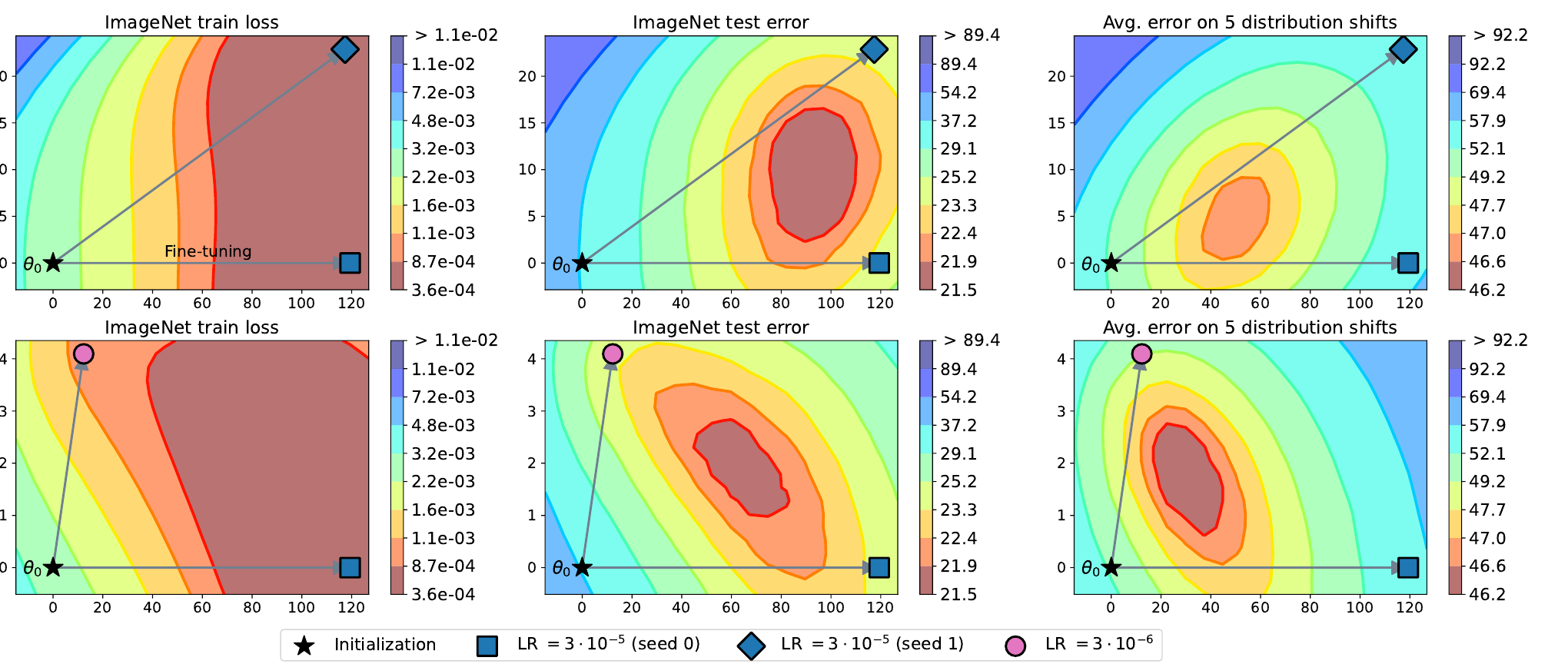
This figure explains why soup can help. The authors fine-tune twice from zero-shot CLIP, use the starting point and two endpoints to span a plane, and plot loss and error on that plane.
In the left column, both fine-tuned solutions already lie in regions of low training loss. The test-error surfaces in the middle and right columns look different: their contours form a basin whose minimum lies between the two fine-tuned solutions, with none of the three points at the bottom. Fine-tuning moves models toward low training loss, while the lowest test error lies off to the side.
Larger angles, more useful averages
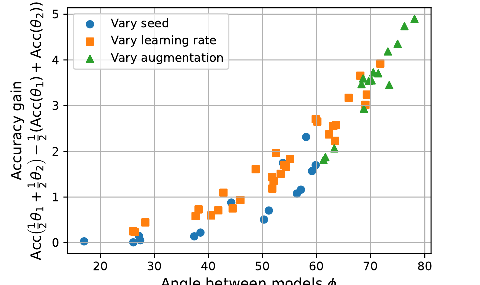
If the best point lies in between, how large is the benefit? The authors define an “interpolation advantage”:
They then examine its relationship to the angle between the models. Here is the angle between and : with pretrained weights as the origin, how differently do the two fine-tuning runs move?
The points roughly trace an upward curve. Blue points that vary only the seed mostly lie near the lower left, with smaller angles and smaller benefits. Changing learning rates or augmentation tends to produce larger angles and greater benefits, reaching roughly 5 percentage points.
This also explains why averaging after a hyperparameter sweep can help. More diverse models offer more useful averages, provided they remain in the same basin.
72 CLIP models
The main experiment fine-tunes CLIP ViT-B/32 on ImageNet 72 times with randomly sampled hyperparameters.
These models share a pretrained starting point. In the main setting, a linear probe initializes the classification head before end-to-end fine-tuning. The search varies learning rate from to , weight decay, training duration from 4 to 16 epochs, label smoothing, mixup, and augmentation. It deliberately retains the good and bad models encountered in a normal hyperparameter search, testing how much extra benefit can be recovered afterward.
| Approach | ImageNet | Mean across five shift datasets |
|---|---|---|
| Best individual model | 80.38 | 47.83 |
| Uniform soup, all 72 models | 79.97 | 51.45 |
| Greedy soup | 81.03 | 50.75 |
| Learned soup, layer-wise coefficients | 81.37 | 50.87 |
| Output ensemble of 72 models | 81.19 | 50.77 |
Accuracy (%), compiled from the original Table 3.
Uniform soup underperforms the best individual model on ImageNet but gains more than three percentage points under distribution shift, showing that some members do drag the average down. Greedy soup beats the best individual model on both measures. Its ImageNet accuracy trails the 72-model ensemble by only 0.16 percentage points, with just one inference pass.
This CLIP greedy soup retains only 5 members. Another experiment with ALIGN also selects 5 from 12 candidates. The layer-wise learned soup reaches a slightly higher 81.37%, but a learned soup with one global set of coefficients reaches 80.89%, below greedy soup. A greedy output ensemble can reach 81.90% on ImageNet, while its shift average is 49.44%. Method rankings change with the model-selection objective; the best column alone cannot capture the full benefit.
The authors also compare soups and ensembles of two models. At moderate learning rates, their accuracies are highly correlated. Ensembling is usually slightly better on ImageNet, while soup is slightly better under distribution shift. At excessively high learning rates, the two models move too far apart and ensembling clearly outperforms soup.
The record-setting pot
The result that attracted the most attention uses ViT-G/14, pretrained on Google's JFT-3B. The authors fine-tune it 58 times on ImageNet, and greedy soup selects 14 members:
| Model | ImageNet | Mean under distribution shift |
|---|---|---|
| CoAtNet-7, the previous record | 90.88 | – |
| ViT-G, best individual model in the sweep | 90.78 | 84.68 |
| ViT-G, greedy soup | 90.94 | 85.02 |
Top-1 accuracy (%), compiled from the original Table 1.
The 90.94% score set the ImageNet record at the time, with 25% less inference computation than CoAtNet-7. Relative to the best model in the hyperparameter search, the gain is 0.16 percentage points without any additional training budget.
Where it works
The authors also test ALIGN, BASIC, two WILDS datasets, and four GLUE text-classification tasks with BERT and T5. Image-classification trends are consistent. Text classification also improves, though less clearly, and the authors treat those results as preliminary.
The text experiments randomly search 32 fine-tuning configurations per task, varying learning rate, batch size, epochs, and seed. The four tasks are MRPC for paraphrase detection, RTE for entailment, CoLA for grammatical acceptability, and SST-2 for sentiment. Their metrics differ: MRPC averages accuracy and F1, CoLA uses Matthews correlation, and only RTE and SST-2 use accuracy. BERT-base improves from 61.0 to 61.7 on RTE and from 92.5 to 93.0 on SST-2, with no gain on MRPC or CoLA; T5-base improves from 78.3 to 79.1 on RTE. These results support merging models fine-tuned for the same task. A single soup solving all four different tasks is outside this experiment.
The authors also state two limitations. First, most experiments use models pretrained on large, diverse datasets. Greedy soup still helps models pretrained on ImageNet-22k, but by much less. Second, ensembling improves calibration, making confidence estimates more accurate; soup does not show that benefit.
For the calibration comparison, they use 20 models differing only in random seed, separating this question from hyperparameter differences, and measure expected calibration error. More accurate classifications and more reliable predicted probabilities are separate requirements. If deployment uses probability thresholds to abstain, the latter needs direct evaluation.
Why can an ensemble still win within the same basin?
Beyond the geometric intuition above, the paper analyzes the cross-entropy difference between soup and logit ensembling. For interpolation between two models, the approximation contains two terms. One involves the second derivative of loss along the line; the other is the variance of the endpoint logit difference under the soup's softmax distribution.
When curvature along the line favors soup, the first term lowers its relative loss. The second favors output ensembling. If the models are already very similar, their logit difference is small; if the soup is already confident and its softmax is concentrated on one class, the variance term is also small. This explains why sharing a basin alone cannot predict the gap between the two methods.
The approximation assumes logits are close to linear along the line. After excluding models trained at , which move too far apart, the authors find a stronger relationship between the approximation and the actual loss difference. In the landscape comparison at a learning rate of , a clear barrier appears between the fine-tuned endpoints. Greedy checks are useful precisely because even a shared starting point can produce such poor ingredients.
Conclusion
Model soups replace “sweep hyperparameters and keep one” with “sweep hyperparameters and average a selected subset.” Training cost stays the same, inference still uses one model, and both CLIP and ViT-G outperform selection of the best individual model.
The conditions resemble WiSE-FT: all members start from the same pretrained weights and should preferably remain in the same basin. Greedy soup's validation check filters out members that have wandered away.
If you already have a collection of models fine-tuned from the same base with different hyperparameters, try this recipe before keeping only the best one.