Original paper
Averaging Weights Leads to Wider Optima and Better Generalization
- Publication
- UAI 2018Conference
- First submitted to arXiv
- arXiv:1803.05407
Cite this paper · BibTeX
The citation identifies the linked source version. It cites the original paper and its authors.
@misc{modelmergingswa2018,
  title = {{Averaging Weights Leads to Wider Optima and Better Generalization}},
  author = {Pavel Izmailov and Dmitrii Podoprikhin and Timur Garipov and Dmitry Vetrov and Andrew Gordon Wilson},
  year = {2018},
  eprint = {1803.05407},
  archivePrefix = {arXiv},
  url = {https://arxiv.org/abs/1803.05407}
}
In late February 2018, Garipov, Izmailov and colleagues published their mode-connectivity paper, including Fast Geometric Ensembling (FGE). Near the end of training, they switch to short learning-rate cycles and save weights whenever the rate reaches its minimum. At inference, they run all saved models and average their outputs.
FGE obtains a useful ensemble within one model's training budget, but every member must still run at inference.
Two weeks later, the same group posted this paper. Looking at FGE samples in parameter space, they found them scattered around the edge of a good region, leaving its center empty.
Average the weights directly and move to the center.
Defining the problem
Averaging an SGD trajectory is an old idea. In convex optimization, Ruppert (1988) and Polyak and Juditsky (1992) analyzed how iterate averaging accelerates convergence. Neural-network practitioners also maintain exponential moving averages (EMA) with decaying learning rates. In the authors' tests, that EMA converges to performance similar to ordinary SGD.
The learning rate is the issue. With continual decay, SGD converges toward one point. Averaging mostly smooths that trajectory and changes little.
The authors want SGD to explore a good region before averaging, and to understand why its mean should generalize better.
Solving the problem
The algorithm
SWA has a short procedure:
- Train with a standard learning-rate schedule, for roughly 75% of the budget in the paper.
- Continue with either a constant rate or cycles that decrease linearly from to .
- At intervals of iterations, incorporate the current weights into the running mean. With a cyclical learning rate, is one cycle, placing samples at the minimum learning rate:
- At the end, use as the final model.
Step 3 computes an incremental arithmetic mean. counts samples already collected. Starting at zero, the first sample becomes the mean; adding the second gives each half the weight. When adding the third, multiply the old mean by and the new sample by , leaving each original sample with weight . Individual checkpoints need no separate storage. This differs from EMA, which favors recent samples.
The learning-rate cycle deserves care. Within each cycle, SWA only decreases linearly, then jumps straight back to the upper bound:
FGE's triangle also rises gradually. SWA omits that half because only the final average needs strong performance; intermediate snapshots may be weaker. A constant rate can explore farther and produce weaker individual points while still giving a good mean.
In the paper's CIFAR setup, VGG and WRN use a constant SWA rate of 0.01. Preactivation ResNet uses 0.01 on CIFAR-10 and 0.05 on CIFAR-100, sampling once per epoch. PyramidNet uses three-epoch cycles from 0.05 to 0.001. These choices are architecture-specific; select the start and rate with your own validation data.
Recompute BatchNorm statistics
An easy detail to miss: BatchNorm's accumulated means and variances correspond to individual checkpoints, rather than . After training, the authors run over the training data in an extra forward pass to collect matching statistics.
PyTorch later added incremental averaging and statistics recomputation to torch.optim.swa_utils. Consider a tiny network with a linear layer and BatchNorm. Two snapshots have linear weights equal to one and three times the identity matrix:
import torch
from torch import nn
from torch.utils.data import DataLoader
from torch.optim.swa_utils import AveragedModel, update_bn

model = nn.Sequential(nn.Linear(2, 2, bias=False), nn.BatchNorm1d(2))
swa_model = AveragedModel(model)
with torch.no_grad():
    for scale in [1.0, 3.0]:
        model[0].weight.copy_(scale * torch.eye(2))
        swa_model.update_parameters(model)

print("平均權重:", swa_model.module[0].weight.tolist())
print("重算前的均值:", swa_model.module[1].running_mean.tolist())
loader = DataLoader(torch.tensor([[1., 2.], [3., 4.]]), batch_size=2)
update_bn(loader, swa_model)
print("重算後的均值:", swa_model.module[1].running_mean.tolist())
平均權重: [[2.0, 0.0], [0.0, 2.0]]
重算前的均值: [0.0, 0.0]
重算後的均值: [4.0, 6.0]
The averaged linear layer is . Its two inputs reach BatchNorm as and , so their mean should be . Averaging learnable parameters alone leaves the running mean at its old value of ; update_bn aligns it with the new weights. This demonstrates statistics updates only; no classifier is trained.
During SWA training, continue gradient updates on the original model as usual, and call update_parameters at the chosen sampling interval. After all averaging, run update_bn once, then switch to eval() for evaluation. Reestimation uses training inputs, with no labels or backpropagation.
Why weight averaging resembles ensembling
FGE averages outputs; SWA averages weights. When are they similar? The authors use a first-order expansion.
Let FGE samples be , their mean and their deviations , so . Expand the network output around :
Averaging over makes the first-order terms sum to , leaving second-order terms:
If the points are sufficiently close, the output ensemble and averaged-weight model differ only by a second-order quantity. FGE deliberately collects points with small moves, allowing SWA to approximate its ensemble with one model.
The argument also requires to be sufficiently smooth nearby, with small second-order remainders. Far-apart models, especially from different random initializations, can have large , making this expansion inadequate to justify similar averaged outputs and averaged weights. SWA collects points from the late part of one training trajectory.
On CIFAR-100 with ResNet-164, the authors run 20 FGE epochs. Adjacent snapshots' class-probability vectors have mean difference norm 0.126; SWA versus the FGE ensemble gives 0.079. Adjacent snapshots agree on predicted classes at most 87.33% of the time, while SWA and the ensemble agree on 95.26%. These observations support the first-order cancellation argument, while retaining a measurable output gap.
Discussion
SGD at the edge
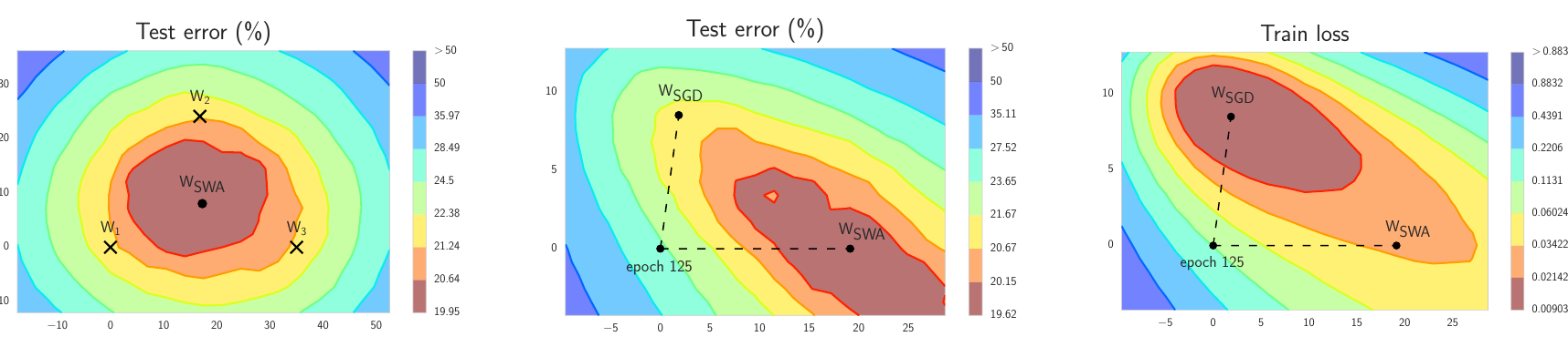
The network is Preactivation ResNet-164 on CIFAR-100. On the left, the motivation is visible: three FGE samples surround the red region, while their mean lies inside.
Read the middle and right together. Both start from the same epoch-125 weights and finish with SGD or SWA. In the training-loss panel, lies within the low-loss region but near its edge. In the test-error panel, is closer than to the minimum-error area.
The training-loss and test-error landscapes are offset. Near the edge of the low-loss region, a small shift in landscape can raise test error; the center provides more room.
Two experiments support this account. First, move outward from both solutions along ten random directions. Distance is horizontal; test error is on the left and training loss on the right. Blue is SWA, green SGD, with one curve per direction.
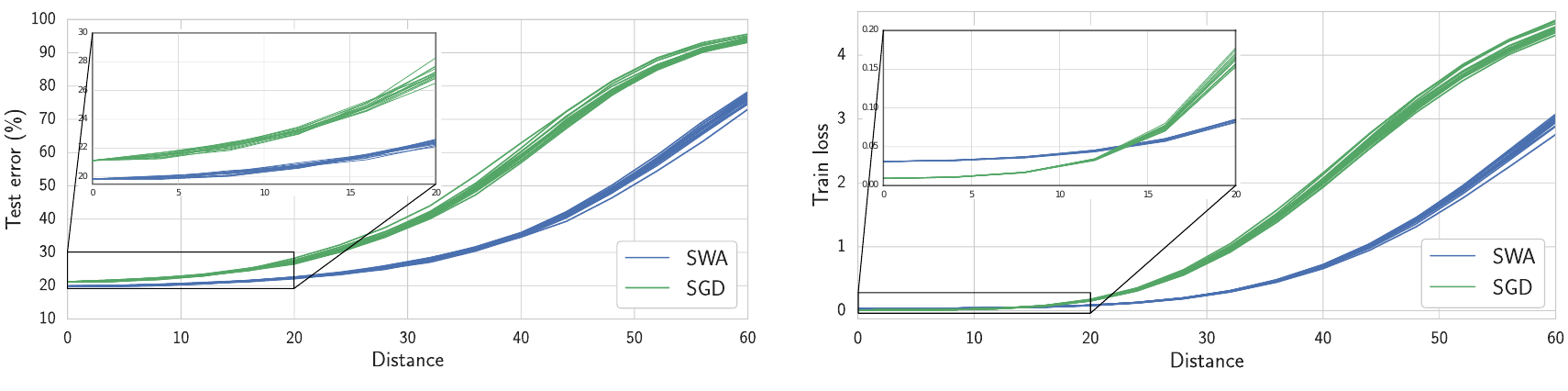
At distance zero, training losses are similar, with SGD slightly lower. SWA's curves are much wider: traveling farther is necessary to raise error by the same amount. These slices measure sensitivity to moving away from each solution.
The second experiment follows the line from to . Training loss and test error are visibly offset. lies on the boundary of a flat region beside a steep slope. The authors conclude that SWA and SGD share a basin, but SWA finds a flatter position within it. Its training loss is often slightly higher; strictly speaking, that position need not be a local loss minimum.
CIFAR and ImageNet
CIFAR experiments use a normal schedule for roughly 75% of the budget and SWA for the remainder. On CIFAR-100, Preactivation ResNet-164 reaches 78.49% with standard SGD and 79.77% with equal-budget SWA, almost matching FGE's 79.84% with one inference model. At 1.5× budget, SWA reaches 80.35%. VGG-16 rises from 72.55% to 73.91%; WRN-28-10 from 80.82% to 81.46%. SWA Table 1
For ImageNet, the authors start from torchvision pretrained models and add five or ten epochs with cyclical learning rates:
| Model | SGD | SWA 5 epochs | SWA 10 epochs |
|---|---|---|---|
| ResNet-50 | 76.15 | 76.83 ± 0.01 | 76.97 ± 0.05 |
| ResNet-152 | 78.31 | 78.82 ± 0.01 | 78.94 ± 0.07 |
| DenseNet-161 | 77.65 | 78.26 ± 0.09 | 78.44 ± 0.06 |
Top-1 accuracy (%), compiled from original Table 2.
All three architectures gain 0.6–0.9 percentage points with a small fraction of their original training cost.
Read budgets and flatness separately
The equal-budget comparison applies to VGG, ResNet and WRN. PyramidNet and Shake-Shake first finish a full standard training budget, then add 0.25 or 0.5 budgets of SWA, so the paper omits their results. CIFAR-100 PyramidNet-272 improves from SGD's 83.41% to at 84.16%. CIFAR-10 Shake-Shake improves from 96.93% to at 97.16%, while gives 97.12%. More averaging and training have diminishing returns.
Extra costs include one stored running-average weight set, a parameterwise weighted update per sample, and a final BatchNorm forward pass. Deployment retains only the averaged model, restoring the original parameter count and per-inference computation. The authors find modest memory overhead for activation-heavy image training. When weights dominate memory, the extra copy needs separate assessment.
Return to flatness. The paper measures ten random directions in a chosen parameterization and the specific SGD–SWA direction, whose SGD neighborhood is steep on one side and flatter on the other. Rescaling network parameters can change the apparent landscape width, so the authors discuss the controversy over flatness as a generalization explanation. Their evidence supports this geometric account for the tested architectures and schedules. Validation accuracy still needs direct measurement.
Conclusion
SWA keeps the late-stage learning rate relatively high, averages visited weights, then recomputes BatchNorm statistics. The intuition is simple: SGD settles near the edge of a good region, and averaging moves the model toward its center.
The last step is easy to forget. If the network uses BatchNorm, run update_bn after averaging so the statistics match the averaged weights.
This average traveled far: when Llama 3's 2024 report discusses post-training model averaging, this paper is its first citation.