Original paper
Linear Mode Connectivity and the Lottery Ticket Hypothesis
- Publication
- ICML 2020Conference
- First submitted to arXiv
- arXiv:1912.05671
Cite this paper · BibTeX
The citation identifies the linked source version. It cites the original paper and its authors.
@misc{modelmerginglinearmodeconnectivity2019,
  title = {{Linear Mode Connectivity and the Lottery Ticket Hypothesis}},
  author = {Jonathan Frankle and Gintare Karolina Dziugaite and Daniel M. Roy and Michael Carbin},
  year = {2019},
  eprint = {1912.05671},
  archivePrefix = {arXiv},
  url = {https://arxiv.org/abs/1912.05671}
}
Even with fixed initial weights and hyperparameters, two training runs differ. Each epoch shuffles data differently, and augmentations sample different crops and flips. The paper calls this randomness SGD noise.
MIT's Jonathan Frankle and Michael Carbin, Element AI's Gintare Karolina Dziugaite, and Daniel Roy of the University of Toronto and Vector Institute ask how much this noise changes. Do two runs approximate one solution, or reach different valleys?
Frankle and Carbin introduced the lottery ticket hypothesis in 2018. They found sparse subnetworks in small networks that train from initialization to full-network accuracy, but had trouble scaling that finding to ImageNet. The second half of this paper uses the same analytical tool to explain why.
Defining the problem
The tool is instability analysis.
Take network at state . This may be its random initialization or its state after training steps, . Duplicate it and train both copies to completion with different SGD noise, obtaining and . Then compare the two weight sets.
Interpolate along their straight segment:
is classification error. The highest error along the segment minus the mean endpoint error defines the error barrier:
A near-zero barrier indicates linear mode connectivity and a state stable to SGD noise. The authors use a two-percentage-point threshold and sample at 30 equally spaced values. Each setting averages nine comparisons: three initializations, each with three data orders.
For endpoints with 8% and 10% error and a maximum interpolation error of 45%, the barrier is percentage points. If the maximum is just 10%, the one-point barrier meets the stability threshold. The definition accounts for endpoint errors, so compare the endpoints as well as the midpoint.
The 30 positions discretely approximate the continuous segment. The measured quantity is classification error, distinct from a cross-entropy loss barrier: identical class predictions can have different confidence. “Stable” below always refers to this measurement and threshold.
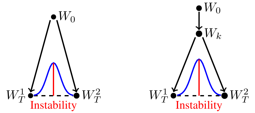
The left branches at initialization; the right shares steps first. Sweep forward from zero to identify when the network settles.
Solving the problem
Branch at initialization
The five networks are LeNet on MNIST, ResNet-20 and VGG-16 on CIFAR-10, and ResNet-50 and Inception-v3 on ImageNet. CIFAR experiments also test lower-learning-rate and warmup variants.
Duplicating at leaves every network except LeNet unstable. Straight-line interpolation raises both training and test error to chance levels. LeNet's error rises by less than one percentage point.
Even from the same initialization, different data orders and augmentations can produce endpoints disconnected by a low-error straight segment. For larger networks, initialization alone is insufficient.
Sweep k
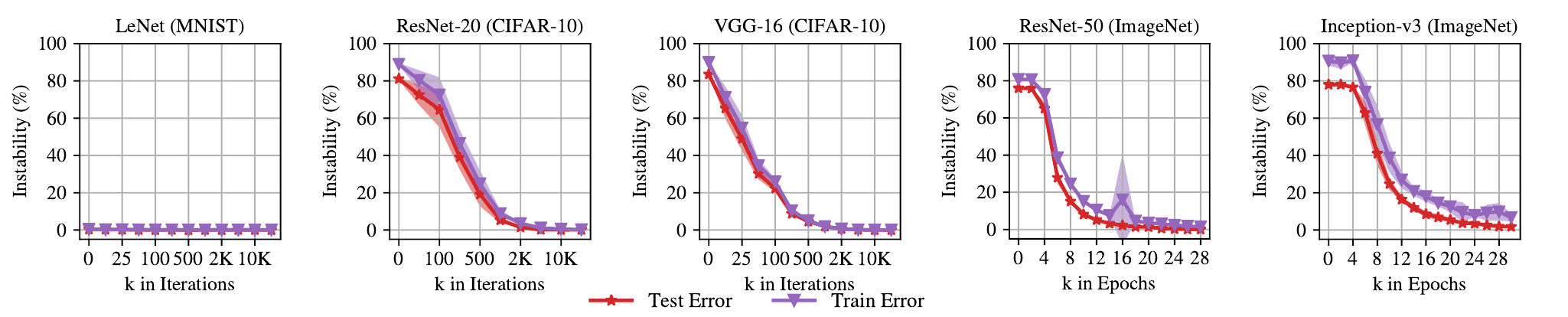
The horizontal axis is training before duplication; the vertical is test instability. Except LeNet, each curve starts high, declines and remains near zero afterward.
The threshold is crossed early: iteration 2,000 for ResNet-20 and 1,000 for VGG-16, just 3% and 1.5% of training. ImageNet takes longer: epoch 18 for ResNet-50 (20%) and epoch 28 for Inception-v3 (16%).
Afterward, sampled data-order and augmentation choices lead to linearly connected regions. These are observations across multiple runs; thresholds depend on architecture, schedule and evaluation data.
| Full network | Total training | First test instability below 2% |
|---|---|---|
| LeNet/MNIST | 24,000 updates | Stable from initialization |
| ResNet-20/CIFAR-10 | 63,000 updates | Around update 2,000, 3% |
| VGG-16/CIFAR-10 | 63,000 updates | Around update 1,000, 1.5% |
| ResNet-50/ImageNet | 90 epochs | Around epoch 18, 20% |
| Inception-v3/ImageNet | 171 epochs | Around epoch 28, 16% |
Compiled from original Figure 3 and training settings. These are standard configurations, excluding lower-rate and warmup variants.
On ImageNet, the test barrier can meet the threshold while the training barrier remains higher. ResNet-50 becomes training-stable later; Inception-v3 never does within the scanned range. “Settles at epoch 18” therefore specifically refers to test error.
Less training time, or genuine stability?
There is a possible confound. As increases, the remaining training shrinks, giving copies less opportunity to diverge. Could shorter training explain the lower instability?
A control always trains a full steps after duplication and restarts the learning-rate schedule. Its instability curves almost overlap the original ones for ResNet-20 and VGG-16. Shorter remaining training time therefore fails to explain the observed stability.
The authors also check whether the model has finished learning at branching. At update 2,000, ResNet-20 still has about 25% test error, eventually reaching 8.3%. VGG-16 has about 20% at update 1,000, eventually reaching 6.3%. Parameters remain closer to initialization than to their final values. Substantial training remains: stability describes which linearly connected region later training will enter, while accuracy continues to improve.
Discussion
When sparse subnetworks succeed
The second half returns to the lottery ticket hypothesis.
Its evidence uses iterative magnitude pruning (IMP): train, prune the smallest-magnitude weights, reset survivors to their initial values, and retrain. Repeat to reach the target sparsity. For the two ImageNet networks, one-shot pruning saves computation. A subnetwork that reaches full-network accuracy is called “matching.”
IMP finds matching subnetworks for LeNet, but fails under standard ResNet-20 and VGG-16 settings and on ImageNet. Retaining 30% of ResNet-50 weights, the full network reaches 76.1%; an IMP subnetwork reset to initialization reaches just 73.7%, similar to random pruning.
Instability analysis aligns with those results: subnetworks matching from initialization are stable from initialization; those failing to match are unstable.
Since full networks become stable after some early training, what if pruning rewinds to step instead of initialization? Previously nonmatching subnetworks then become matching, at nearly the same points where they become stable. ResNet-50 and Inception-v3 IMP subnetworks stabilize at epochs 5 and 6, much earlier than their full networks' epochs 18 and 28.
This extends the lottery-ticket observation to ImageNet, with the ticket found in early training rather than initialization.
Which weights are rewound?
An operational description helps. Save the full network's step- weights and use binary mask to mark survivors. Each round trains from to completion, updates using final magnitudes, prunes the smallest 20% of currently surviving weights, then rewinds to the same . After two rounds, the retained fraction is ; each round removes 20% of the survivors, rather than 20% of the original network.
The mask is chosen using trained endpoints, requiring multiple training runs. The experiment establishes useful subnetworks in early weights. Real training-time savings also depend on the cost of finding masks and hardware support for sparse computation.
Controls separate structure from weights: one randomly prunes while preserving IMP's layerwise retention fractions; another uses the IMP mask with newly randomized surviving weights. At the selected extreme sparsities, most such random subnetworks remain unstable and less accurate even with later rewinding.
Standard ResNet-20 retaining 16.8% stabilizes under IMP around update 500; VGG-16 retaining 1.5% around update 1,000. Both ImageNet networks retain 30%, stabilizing at epochs 5 and 6. Sparse subnetworks can stabilize before full networks; stability has no simple monotonic relationship with parameter count.
Stable can still be too small
Increasing CIFAR-10 sparsity, the authors find matching IMP subnetworks when ResNet-20 retains roughly 80.0–13.4% of weights, and VGG-16 roughly 16.8–1.2%. Below those ranges, even IMP finds no matching subnetwork across the tested rewinding times.
Here, cross-sparsity analysis allows a roughly 0.2-percentage-point accuracy drop for matching. At extreme sparsity, stability still accompanies lower error, but capacity is insufficient to match the full network. Stability is strongly associated with successful training; treating it as sufficient for every subnetwork would go too far.
The appendix also compares endpoints using distance, cosine distance, prediction disagreement and per-example loss differences. Full-network parameter distances decrease smoothly with later branching, without suddenly reaching zero at stability. Endpoints in one region can remain far apart. Interpolation additionally tests whether the entire intervening segment works, something endpoint distance alone leaves unanswered.
Implications for merging
The paper studies a basic prerequisite for direct weight averaging, even though model merging is outside its explicit topic.
Its copies share data and hyperparameters and differ only in SGD noise. After their shared early training phase, straight interpolation avoids an error barrier, allowing their average to stay in the low-loss region.
Later pretraining-plus-fine-tuning workflows provide a much longer shared history and a useful starting point for merging. Their different fine-tuning data and objectives extend beyond this paper's SGD-noise-only experiment. Later research and measured interpolation curves must establish whether they can be added.
Conclusion
This paper turns the question of shared solution valleys into a measurable one. Except for the smallest network, branching at initialization fails the criterion; sharing the first 1.5–20% of training lets the tested endpoints become linearly connected.
The same tool extends the lottery-ticket findings: settings without useful initialization-reset subnetworks gain them by rewinding to early trained weights.
Before directly averaging two models, ask when they last shared a training path.