Original paper
Loss Surfaces, Mode Connectivity, and Fast Ensembling of DNNs
- Publication
- NeurIPS 2018Conference
- First submitted to arXiv
- arXiv:1802.10026
Cite this paper · BibTeX
The citation identifies the linked source version. It cites the original paper and its authors.
@misc{modelmergingmodeconnectivity2018,
  title = {{Loss Surfaces, Mode Connectivity, and Fast Ensembling of DNNs}},
  author = {Timur Garipov and Pavel Izmailov and Dmitrii Podoprikhin and Dmitry Vetrov and Andrew Gordon Wilson},
  year = {2018},
  eprint = {1802.10026},
  archivePrefix = {arXiv},
  url = {https://arxiv.org/abs/1802.10026}
}
Train the same network with two random seeds and you get very different weights, often with similar accuracy.
Those weight sets are two points in parameter space. Join them with a straight line and evaluate a few points along it: the middle often has alarmingly high error. The paper's VGG-16 example on CIFAR-10 reaches 90% test error at the midpoint—chance performance across ten classes.
It is natural to picture each solution as an isolated valley, separated from others by high mountains.
Garipov, Izmailov, Podoprikhin, Vetrov and Wilson, from Samsung's Moscow AI Center, Skoltech, Cornell and HSE, ask a different question: if a straight road fails, what about a curved one?
Defining the problem
Let and be two independently trained networks' weights, and the training loss. The straight connection is
The goal is a curve with endpoints fixed at and . Parameters control its shape, and loss should stay low along the whole curve.
Finding one would change the picture of isolated solution valleys. Failure would require distinguishing a restrictive curve family, unsuccessful optimization and genuinely hard-to-connect endpoints. One failed search cannot rule out other paths.
Solving the problem
Let the curve learn
Every point on the curve supplies network weights whose loss can be evaluated. The objective averages loss along the curve:
Sampling estimates the gradient of this expectation. At each step, use as the sampling range and draw uniformly. Construct that point's weights, evaluate loss on a minibatch, and take a gradient step on . The endpoints , stay fixed; only the curve-shaping parameters learn.
Two curve families
The authors use two simple parameterizations. First is a polygonal chain with one bend, located at :
Second is a quadratic Bézier curve, where is the control point:
Both curves reach the fixed endpoints at , . has exactly the same shape as the network weights, so the number of learned parameters equals one network's parameter count.
Consider the Bézier midpoint. At , each endpoint contributes and the control point contributes . Moving the control point one unit therefore moves the midpoint weights half a unit. During backpropagation, the control-point gradient is the current weight gradient multiplied by . Endpoint weights stay outside the optimizer, preserving the original models.
The polygonal chain works similarly, with the multiplier changing between its two halves. Curve training reuses ordinary forward and backward passes; the main extra operation is a linear weight combination. It still requires training data, additional optimization and storage for one control point. Finding a low-loss path comes with these costs.
Try a small network
A small network makes the effect visible. Use scikit-learn's 1,797 handwritten 8×8 digits and an MLP with two 200-unit hidden layers. Train two endpoints on the same 1,200 images with different initial weights, then initialize a Bézier control point at the straight-line midpoint:
import torch
import torch.nn as nn
from torch.func import functional_call
from sklearn.datasets import load_digits

X, y = load_digits(return_X_y=True)
X = torch.tensor(X / 16.0, dtype=torch.float32)
y = torch.tensor(y)
perm = torch.randperm(len(X), generator=torch.Generator().manual_seed(0))
idx_train, idx_test = perm[:1200], perm[1200:]

def make(seed):
    torch.manual_seed(seed)
    return nn.Sequential(nn.Linear(64, 200), nn.ReLU(),
                         nn.Linear(200, 200), nn.ReLU(),
                         nn.Linear(200, 10))

def train(model, seed, steps=480):
    opt = torch.optim.SGD(model.parameters(), lr=0.1)
    g = torch.Generator().manual_seed(seed)
    for _ in range(steps):
        b = idx_train[torch.randint(len(idx_train), (50,), generator=g)]
        loss = nn.functional.cross_entropy(model(X[b]), y[b])
        opt.zero_grad(); loss.backward(); opt.step()
    return {k: v.detach() for k, v in model.state_dict().items()}

w1 = train(make(1), seed=10)                 # 兩個端點:同樣的資料,不同的初始權重
w2 = train(make(2), seed=20)
net = make(0)

@torch.no_grad()
def evaluate(w):
    loss = nn.functional.cross_entropy(functional_call(net, w, (X[idx_train],)), y[idx_train]).item()
    acc = (functional_call(net, w, (X[idx_test],)).argmax(1) == y[idx_test]).float().mean().item()
    return f"loss {loss:.3f}, 測試 {acc:.1%}"

def line(t):
    return {k: (1 - t) * w1[k] + t * w2[k] for k in w1}

theta = {k: v.clone().requires_grad_(True) for k, v in line(0.5).items()}   # 彎點從直線中點出發

def bezier(t):
    return {k: (1 - t) ** 2 * w1[k] + 2 * t * (1 - t) * theta[k] + t ** 2 * w2[k] for k in w1}

opt = torch.optim.SGD(theta.values(), lr=0.1)
g = torch.Generator().manual_seed(0)
for _ in range(1200):
    t = torch.rand((), generator=g).item()   # 每一步隨機抽一個 t
    b = idx_train[torch.randint(len(idx_train), (50,), generator=g)]
    loss = nn.functional.cross_entropy(functional_call(net, bezier(t), (X[b],)), y[b])
    opt.zero_grad(); loss.backward(); opt.step()   # 只更新彎點 theta,端點不動

for t in [0, 0.25, 0.5, 0.75, 1]:
    print(f"t={t:<4}  直線: {evaluate(line(t))}  |  曲線: {evaluate(bezier(t))}")
t=0     直線: loss 0.119, 測試 95.5%  |  曲線: loss 0.119, 測試 95.5%
t=0.25  直線: loss 0.415, 測試 93.6%  |  曲線: loss 0.142, 測試 95.5%
t=0.5   直線: loss 0.949, 測試 88.9%  |  曲線: loss 0.156, 測試 95.3%
t=0.75  直線: loss 0.420, 測試 95.0%  |  曲線: loss 0.140, 測試 95.3%
t=1     直線: loss 0.119, 測試 94.8%  |  曲線: loss 0.119, 測試 94.8%
functional_call lets one network structure evaluate externally supplied weights, including any point on the curve. Both endpoints have loss 0.119. The straight midpoint reaches 0.949; the learned curve's midpoint reaches just 0.156 and keeps test accuracy around 95%.
This is a tiny network with a modest straight-line barrier. The paper's larger networks have much higher walls.
Discussion
Curves in larger networks
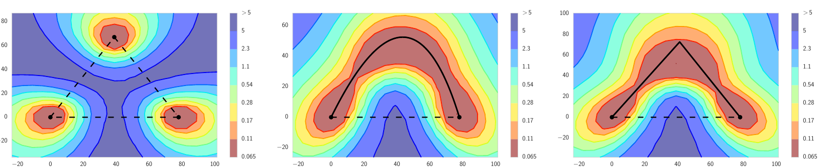
This figure shows ResNet-164 training loss on CIFAR-100. Each panel slices parameter space in two dimensions, with its horizontal axis passing through two solutions. Red means low loss; blue means high loss.
The left plane is defined by three independently trained solutions, each in its own red region separated by blue, matching the isolated-valley intuition. The middle and right use different planes containing the learned curves. Red channels now connect the lower two solutions, while their straight dashed segment still crosses blue.

Figure 2 plots the same experiment as curves. The red straight segment sends training loss and test error soaring in the left and middle panels; the green Bézier curve and blue polygonal chain remain almost flat.
Barrier height depends on architecture. On CIFAR-10, VGG-16 reaches 90% midpoint test error. ResNet-158 and Wide ResNet-28-10 peak at 80% and 66%. The authors relate this to earlier observations that residual-network landscapes are more regular than those of classical models such as VGG.
The connecting curve is also nonunique. Training two polygonal chains with different seeds between the same VGG-16 endpoints gives bend points 29.6 apart, versus endpoint distance 50.
Points along the curve make different predictions
If loss stays low along the curve, could its points merely be different parameterizations of the same model?
The right panel addresses this. Ensemble the endpoint with a point by averaging their outputs. Along the polygonal chain, ensemble error starts declining at ; by , it matches the ensemble of the independently trained endpoints. Moving only a short distance yields a model with meaningfully different predictions and high accuracy.
If curve points represented the same function—for example, by reciprocal rescaling around ReLU—the ensemble would gain nothing. The appendix constructs such unhelpful connecting curves too.
From curves to ensembles
This observation leads to the paper's second contribution: Fast Geometric Ensembling (FGE).
If a small move near one solution finds a different, useful model, explicitly learning a connecting curve becomes unnecessary. FGE trains with a standard learning-rate schedule for roughly 80% of the budget, then uses short cycles of two to four epochs. High rates move outward; low rates return toward the basin floor. Save weights at the low point of each cycle and ensemble the resulting models.
Compared with Snapshot Ensembles, the distinction is step size. Snapshot Ensembles uses 20–40-epoch cycles throughout training; FGE uses short cycles only near the end. On CIFAR-100 with Preactivation-ResNet-164, successive FGE checkpoints are about 7 apart in Euclidean parameter distance, versus about 40 for Snapshot Ensembles.
The ImageNet result is straightforward. Starting from pretrained ResNet-50 at 23.87% top-1 error, five extra FGE epochs with two-epoch cycles produce a four-model ensemble, including the original, at 23.31%: a reduction of 0.56 percentage points.
FGE still runs every ensemble member during inference.
The cycle and checkpoint timing
Read the original figure's left side from top to bottom: learning rate, test error and parameter distance from the start. Black circles mark saved checkpoints. The right compares results under equal training budgets: crosses are individual snapshots; connected diamonds are ensembles.
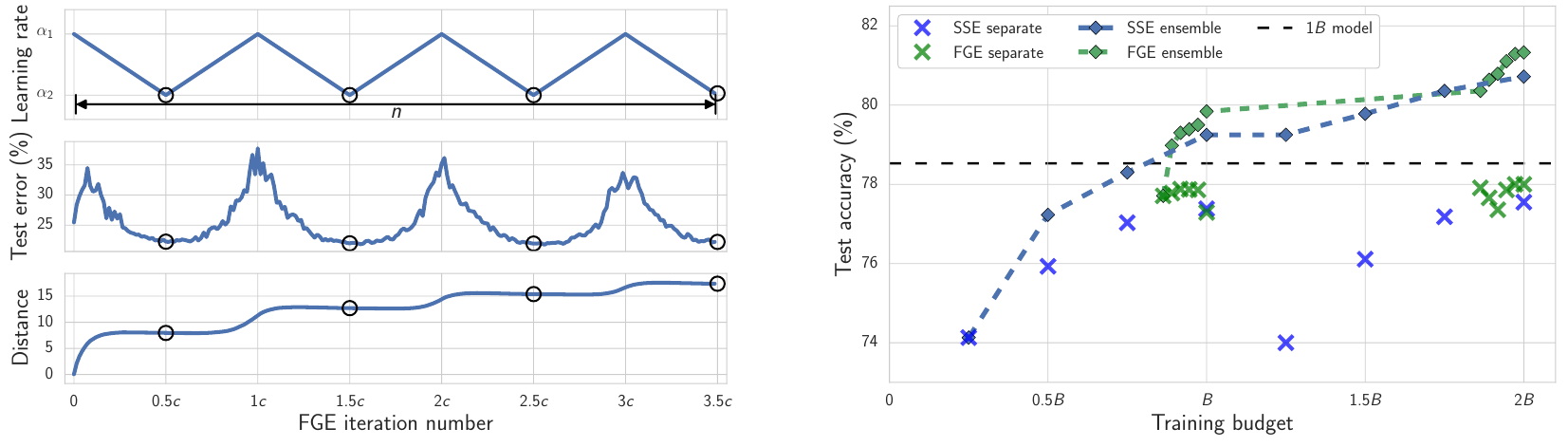
FGE uses a triangular learning rate. Let a cycle contain an even number of minibatch updates, with within-cycle position and bounds :
The rate falls from high to low, then rises again. Checkpoints are saved halfway through the cycle, at when the learning rate equals . Error temporarily rises near the high-rate phase; the desired snapshots have returned to a low-error region.
In the CIFAR experiments, VGG uses two-epoch cycles with , ; ResNet and WRN use four-epoch cycles with , . For example, with ResNet's standard budget of epochs, the normal schedule runs through epoch 125, then six models are collected over epochs 126–147. The snapshots share the earlier trajectory, saving repeated training from scratch.
This clarifies the roles of curve search and FGE. Curve search fixes two endpoints and trains a bend to test whether a low-loss channel exists. FGE starts from one model and uses short cycles to collect nearby solutions. Running FGE requires neither a second independently trained endpoint nor a learned Bézier curve.
Accuracy under the same budget
Separate training budget from the number of models used at inference. The paper's is the epoch budget for training one conventional model to convergence; doubles that budget. The table selects CIFAR-100 results at ; its metric is test error, where lower is better.
| Architecture | Independent training (Ind) | Snapshot Ensembles | FGE |
|---|---|---|---|
| VGG-16, | 27.4 ± 0.1 | 26.4 ± 0.1 | 25.7 ± 0.1 |
| Preactivation ResNet-164, | 21.5 ± 0.4 | 20.9 ± 0.2 | 20.2 ± 0.1 |
| WRN-28-10, | 19.2 ± 0.2 | 17.9 ± 0.2 | 17.7 ± 0.2 |
Test error (%), compiled from original Table 1. Each row uses the same training budget, while inference model counts vary by method.
All three beat Snapshot Ensembles, with reductions of 0.7 percentage points for both VGG and ResNet. At , CIFAR-100 WRN scores are Ind 17.48%, SSE 17.30%, FGE 16.95%. But for CIFAR-10 WRN at , Ind reaches 3.31% and FGE 3.52%. Advantages vary with dataset, architecture and budget.
The authors also measure prediction diversity. On CIFAR-100 with ResNet-164, independently trained models disagree on 19.97% of test images, versus 14.57% for two snapshots from one FGE run. Individual FGE snapshots are slightly weaker too: about 78.0% accuracy versus 78.5% for full independent training. FGE's advantage is collecting more useful snapshots in the same time, offsetting those per-model and diversity deficits.
Finally, BatchNorm matters. Changing weights also changes intermediate activation distributions. The appendix reestimates BatchNorm statistics before evaluating loss along the curve. Reusing endpoint running means and variances can mix statistics mismatch into the apparent barrier. Ensure each point's network can infer correctly before interpreting the landscape.
Conclusion
A simple training procedure connects independently trained solutions with a one-bend path of nearly constant loss, even when their straight segment crosses a high wall.
The picture of isolated valleys gives way to low-loss channels between solutions, with curved paths. Directly averaging independently trained networks can fail because averaging follows the straight segment.
FGE leaves the inference cost of an ensemble. Two weeks later, the same group introduced SWA: average those saved weights into a single model.