Original paper
Editing Models with Task Arithmetic
- Publication
- ICLR 2023Conference
- First submitted to arXiv
- arXiv:2212.04089
Cite this paper · BibTeX
The citation identifies the linked source version. It cites the original paper and its authors.
@misc{modelmergingtaskarithmetic2022,
  title = {{Editing Models with Task Arithmetic}},
  author = {Gabriel Ilharco and Marco Tulio Ribeiro and Mitchell Wortsman and Suchin Gururangan and Ludwig Schmidt and Hannaneh Hajishirzi and Ali Farhadi},
  year = {2022},
  eprint = {2212.04089},
  archivePrefix = {arXiv},
  url = {https://arxiv.org/abs/2212.04089}
}
A pretrained model usually needs some changes before use. Improving it on a task, reducing toxic language, or adapting it to new data all fall under what this paper calls “editing.”
Fine-tuning is the most common editing method. Each run produces another model. To make a model handle two things at once, a common approach combines the two datasets for multitask training. Each added capability calls for another adjustment to the data and training process.
Ilharco, Ribeiro, Wortsman, and colleagues from the University of Washington, Microsoft Research, and AI2 had recently worked on WiSE-FT and Model Soups, both studying linear combinations of weights. Here they take a different angle: isolate “what fine-tuning changed” and manipulate it as a vector.
Defining the problem
Let be pretrained weights and the weights after fine-tuning on task . A task vector is their difference:
The vector is as large as the whole model. It records the direction and distance that every weight moves for task .
We can add a task vector to weights , with a scaling coefficient :
Setting and recovers the fine-tuned model exactly. Held-out validation data determine .
There is a prerequisite. Task vectors subtract weights element by element, so the architecture must stay the same and fine-tuning must add no parameters. The authors therefore choose two kinds of “open-ended” models: open-vocabulary image classifiers such as CLIP, which change tasks by using class names and the text encoder to construct a classification head, and text-to-text language models such as T5 and GPT-2.
Can these vectors be added and subtracted like numbers, with model behavior following along?
Solving the problem
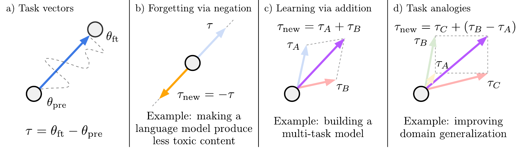
The authors study three elementwise operations:
- Negation, for forgetting: . Move from pretrained weights in the direction opposite to fine-tuning, degrading performance on that task while preserving other tasks as much as possible.
- Addition, for learning: . Add several task vectors to produce a model that handles those tasks together.
- Analogy: if four tasks satisfy “A is to B as C is to D,” use to improve D, even with very little data for D.
All three finish with . Editing consists entirely of vector operations, and inference uses the same memory and computation as the original model.
It is easy to conflate “adding tasks” with “averaging two fine-tuned models.” With and , we have
Direct averaging is task arithmetic with ; retains both full fine-tuning updates. For example, suppose base parameters are and the tasks produce and . Averaging gives , while task addition gives . In a large network, a twofold scale difference can change performance, so coefficient selection is part of the method.
Analogy sounds the most abstract, so consider the paper's example. We want sentiment classification for Yelp reviews, but have sentiment labels only for Amazon reviews and unlabeled text from Yelp. The authors construct:
is learned by sentiment classification on Amazon. The two vectors in parentheses come from language-model training on Yelp and Amazon text respectively, requiring no labels. Their difference roughly describes the domain shift “from Amazon to Yelp.”
Discussion
Negation: forgetting a task
Image-classification experiments use CLIP with eight target datasets: car models in Cars, textures in DTD, satellite imagery in EuroSAT and RESISC45, traffic signs in GTSRB, handwritten digits in MNIST, scenes in SUN397, and house numbers in SVHN. ImageNet is the control task for checking damage to other capabilities.
Subtracting task vectors from ViT-L/14 lowers mean accuracy across the eight target tasks from 64.8% to 19.0%, a 45.8-percentage-point drop. ImageNet falls from 75.5% to 72.9%, a cost of 2.6 percentage points. By comparison, gradient ascent on the target task, pushing its loss upward, also degrades the target but severely damages ImageNet accuracy, to 16.3%. Adding a random vector of equal magnitude has little effect on the target task.
For text generation, the authors fine-tune GPT-2 Large on Civil Comments with toxicity scores above 0.8, creating a task vector for toxic language, then subtract it. The share of generations classified as toxic falls from 4.8% to 0.8%, while WikiText-103 perplexity changes from 16.4 to 16.9. Gradient ascent also reduces toxicity, but makes perplexity unusably poor.
This experiment generates 1,000 passages from a fixed controversial prefix and scores them with the Detoxify classifier. It chooses the largest that worsens perplexity by at most 0.5. The baseline of fine-tuning directly on nontoxic comments gives 1.8% toxicity and 17.2 perplexity, a less favorable tradeoff in this setting. The appendix tests other prompts, RealToxicityPrompts, and different GPT-2 sizes; toxicity on difficult prompts still leaves room for improvement.
Here, “forgetting” refers to measurable behavioral degradation, supported by outputs on specified tasks and prompts. Removing a particular training example or guaranteeing that specific information cannot be extracted requires a form of validation absent from this paper.
Addition: several tasks in one model
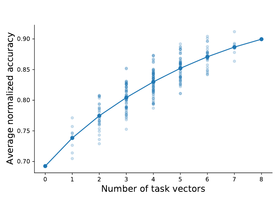
Because tasks vary in difficulty, the authors compare normalized accuracy: merged-model accuracy on each task divided by the accuracy of that task's individually fine-tuned model. A value of 100% matches the separate experts.
Pairwise addition retains an average of 98.9% of expert accuracy on the two corresponding tasks. The figure above uses a different measurement: each point is a subset of vectors, but every score averages across all eight tasks. The authors examine subsets. With no vectors, the zero-shot pretrained model scores roughly 69%; greater task coverage raises the overall average. With all eight vectors available for selection, the best multitask model found reaches 91.2% normalized accuracy.
One model handling eight tasks loses less than a tenth relative to deploying eight separate experts. There is still a merging loss, and preserving everything becomes harder as task count grows.
Normalization divides within each task before averaging. If experts score 80% and 100% on two tasks, and the merge scores 72% and 95%, retention is . Raw mean accuracy is 83.5%; the two measures serve different purposes. The paper's 91.2% measures retention of the separate experts.
The coefficient is searched on validation data from 0 to 1 in steps of 0.05. All added vectors share one , avoiding a combinatorial explosion from separately tuning each task. The appendix finds that 0.3 to 0.5 works well for many combinations, but optima still vary substantially across subsets. Having more vectors available also does not ensure that including every one is best.
One strong baseline also matters. Direct multitask fine-tuning on all eight datasets reaches 99.4% normalized accuracy, above task arithmetic's best 91.2%. Task arithmetic offers modularity, no need to reacquire each task's training data, and training-free merging. When data can be centralized and another training run is feasible, multitask fine-tuning remains a priority comparison.
For natural language, the authors fine-tune T5-base on four GLUE tasks, then collect 427 compatible public models from Hugging Face. They add those task vectors to their models one at a time, choosing the best vector and coefficient on validation data. A vector from someone else's task can sometimes improve the target beyond ordinary fine-tuning.
The four-task mean score rises from 78.1 to 78.6; MRPC rises from 88.5 to 89.3, with other gains around 0.2 to 0.7. This is the result of searching many candidates and selecting a helpful vector. The appendix also merges pairs from six public T5 checkpoints covering question answering, summarization, sentiment, and text generation, using accuracy, exact match, or ROUGE-2 as appropriate. One accuracy number cannot summarize all those text tasks.
Analogy: learning without target labels
The Yelp–Amazon example above improves on fine-tuning with Amazon sentiment data alone across several T5 sizes, approaching direct fine-tuning on the target dataset. The authors find that the sentiment vector needs more weight, so use two independent coefficients.
For example, with Amazon as the target, T5-base fine-tuned only on Yelp sentiment labels reaches 90.8%. Domain analogy raises it to 92.7%, compared with 93.2% from fine-tuning on Amazon labels. The two language-model vectors require unlabeled text from both target and auxiliary domains. Even without target labels, the method uses target-domain data. Analogy estimates the domain shift from that unlabeled text and transfers the learned sentiment-classification direction along it.
Another experiment takes 125 classes shared by ImageNet and a hand-drawn sketch dataset, dividing them into four subpopulations: photographs/sketches crossed with two class groups. To improve a subpopulation such as “sketch lions,” it uses
The mean improvement over the pretrained model is 3.4 percentage points, roughly equivalent to collecting and labeling about one hundred additional training examples for the target subpopulation.
Why can the vectors be added?
The authors measure pairwise cosine similarity between CLIP task vectors on nine tasks. Most pairs lie between 0.01 and 0.03, nearly orthogonal. Higher values occur for semantically related tasks. MNIST and SVHN both recognize digits and reach 0.18. GTSRB traffic signs also involve digits, giving 0.06 with those tasks. EuroSAT and RESISC45 both use satellite imagery and reach 0.05.
The authors hypothesize that this near-orthogonality lets the vectors add with little interference. This is an interpretation of the observation. Later analysis by Ortiz-Jimenez and colleagues emphasizes weight disentanglement, a property brought by pretraining and absent in randomly initialized models.
Two further observations help in practice. First, addition degrades faster at higher learning rates and is more sensitive than individual fine-tuning. The authors recommend conservative fine-tuning learning rates when using task vectors. Second, vectors align with their final direction early in fine-tuning. Adding intermediate vectors after only a few hundred steps already brings accuracy close to saturation.
Limitations
The authors' limitations are direct. Task vectors require the same architecture, and every experiment uses models derived from the same pretrained weights.
They also note that this constraint leaves a large practical pool. At the time of writing, Hugging Face already had more than three thousand models fine-tuned from the same BERT-base and more than eight hundred from the same T5-small.
Conclusion
Task arithmetic represents fine-tuning as a vector, then shows that these vectors can be added, subtracted, and used in analogies, with model behavior broadly following those operations.
Training remains ordinary fine-tuning; the new part is how we view its result. Later methods such as TIES-Merging and DARE build on this framework, each addressing interference during vector addition.
The next time you find a Hugging Face model fine-tuned from a familiar base, try subtracting that base and looking at the resulting vector.