Original paper
Robust fine-tuning of zero-shot models
- Publication
- CVPR 2022Conference
- First submitted to arXiv
- arXiv:2109.01903
Cite this paper · BibTeX
The citation identifies the linked source version. It cites the original paper and its authors.
@misc{modelmergingwiseft2021,
  title = {{Robust fine-tuning of zero-shot models}},
  author = {Mitchell Wortsman and Gabriel Ilharco and Jong Wook Kim and Mike Li and Simon Kornblith and Rebecca Roelofs and Raphael Gontijo-Lopes and Hannaneh Hajishirzi and Ali Farhadi and Hongseok Namkoong and Ludwig Schmidt},
  year = {2021},
  eprint = {2109.01903},
  archivePrefix = {arXiv},
  url = {https://arxiv.org/abs/2109.01903}
}
When CLIP first appeared, one of its biggest surprises was its robustness.
Without task-specific fine-tuning on ImageNet labels, it could already perform zero-shot classification using representations learned from image–text pretraining, treating the text vectors for “a photo of a {class}” as a classifier. More unusually, its accuracy dropped much less than that of conventional ImageNet models on variants such as the newly collected ImageNetV2, ImageNet-Sketch, and the artistic renditions in ImageNet-R.
Fine-tuning could undo that robustness. Experiments in the original CLIP paper and BASIC found that fine-tuning on ImageNet greatly improved ImageNet accuracy, while accuracy on several distribution-shift datasets fell below the zero-shot model.
Wortsman, Ilharco, and colleagues from the University of Washington, OpenAI, Columbia, Google, AI2, and other institutions wanted to retain both benefits.
Defining the problem
The paper first introduces a measure called effective robustness.
Plot a collection of conventional ImageNet-trained models, with ImageNet accuracy on the horizontal axis and average accuracy on distribution-shift datasets on the vertical axis. The points lie roughly along a straight line after logit scaling of the axes. Effective robustness measures how far a model sits above that trend:
is the trend line for conventional models. Zero-shot CLIP sits on a higher line and has substantial effective robustness. After fine-tuning, its point moves right as ImageNet accuracy improves, but falls toward the conventional-model trend.
The authors also observe two difficulties during fine-tuning. First, small hyperparameter changes can produce large differences on shifted data. Two learning rates, for example, can differ by only 0.3 percentage points on ImageNet yet by 8 percentage points under distribution shift, and ImageNet performance alone cannot identify the better choice. Second, more aggressive fine-tuning, such as using a higher learning rate, brings larger ImageNet gains alongside larger robustness losses.
Solving the problem
Two steps
WiSE-FT, short for weight-space ensembles for fine-tuning, has just two steps:
- Fine-tune the zero-shot model as usual.
- Linearly interpolate the zero-shot and fine-tuned models in weight space:
gives the zero-shot model, and gives the fine-tuned model. Intermediate values require no further training. The result is a single model with the same inference cost as before.
What about the classification head?
For interpolation to work, every set of weights must correspond across the two models. CLIP's zero-shot classifier is a linear layer . Each column is the text vector for a class description, “a photo of a {class},” and the output is the inner product between the image features and each column.
For end-to-end fine-tuning, the authors initialize the final classification layer with this zero-shot classifier, then train it together with the image encoder. Both models have exactly the same structure and parameter shapes, and share the same starting point, so their weights can be mixed element by element.
The experimental classification head also includes CLIP's learned temperature scale. Class text vectors are constructed by averaging over multiple prompts; ImageNet uses the 80 templates supplied by the original authors. Merging must preserve the same class ordering, feature normalization, and scaling. Checking that both matrices have shape leaves another question to check: does column still denote the same class?
We can work through the LC case explicitly. With image representations fixed:
The right-hand side is the weighted average of two sets of logits. If the two-class scores for an image are and , then gives . Averaging the classification heads first produces the same scores. Applying softmax separately and then averaging probabilities is a different operation.
End-to-end fine-tuning changes , so this distributive identity cannot split the whole network into two outputs. The paper therefore measures weight averaging and output ensembling separately. Both improve robustness; end-to-end weight averaging performs more favorably in the comparison and runs just one encoder, while output ensembling requires two image-encoding passes. In the LC setting, both can share fixed features, so the computational difference lies mainly in the classification heads.
Discussion
Curves on the scatter plot
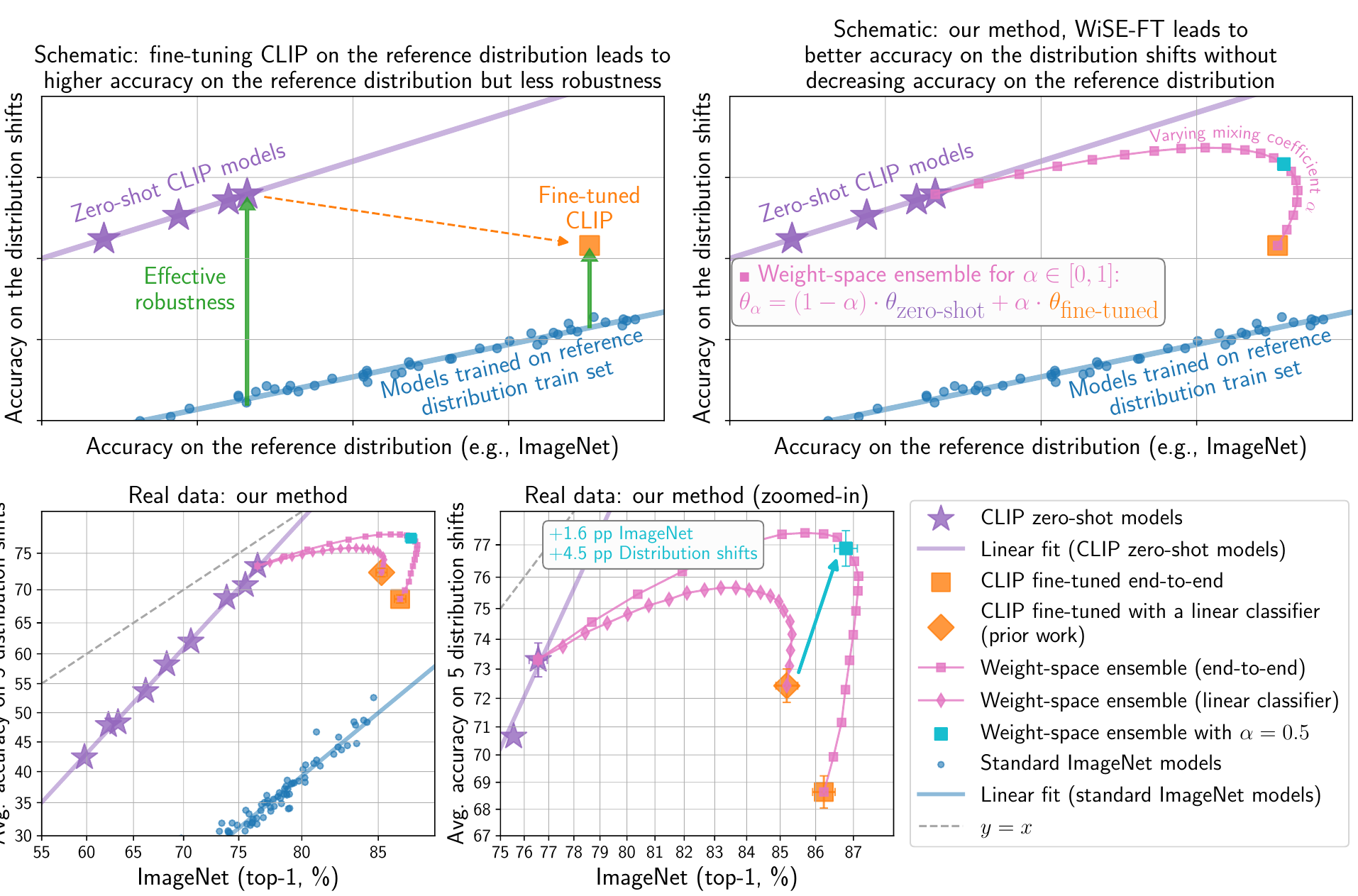
The upper row is schematic. In the left plot, zero-shot CLIP, shown as a purple star, sits above the conventional-model trend line. The green arrow measures effective robustness. Fine-tuned CLIP, the orange square, moves right but falls downward. The right plot shows WiSE-FT: as goes from 0 to 1, pink points trace an upward-bending curve, with an intermediate region both farther right and higher than either endpoint.
The lower row uses real data from ViT-L/14@336px. In the enlarged lower-right plot, pink squares denote interpolated end-to-end models. They start at the purple zero-shot star, bend upward and right, and finally return to the orange fine-tuned square.
The numbers
For the main CLIP ViT-L/14@336px model, results on ImageNet and five derived distribution-shift datasets are:
| Model | ImageNet | Mean across five shift datasets |
|---|---|---|
| Zero-shot, PyTorch reproduction | 76.6 | 73.4 |
| Fine-tuned linear classifier | 85.2 | 72.6 |
| End-to-end fine-tuning | 86.2 | 68.6 |
| WiSE-FT, end-to-end, | 86.8 | 76.9 |
| WiSE-FT, end-to-end, best per column | 87.1 | 77.4 |
Accuracy (%), compiled from the original Table 1. The last row selects separately for each column.
End-to-end fine-tuning raises ImageNet accuracy from 76.6% to 86.2%, while the five-dataset shift average drops from 73.4% to 68.6%. With , WiSE-FT reaches 86.8% on ImageNet, slightly above end-to-end fine-tuning, and 76.9% on shifted data, above even the zero-shot model. Compared with linear-classifier fine-tuning in the original CLIP paper, its gains on shifted datasets are 4 to 6 percentage points.
The five shift datasets test different changes. ImageNetV2 recollects photographs from a similar distribution. ImageNet-R uses renditions such as sculpture and painting and contains only 200 classes. Sketch uses drawings. ObjectNet tests different backgrounds and viewpoints, with 113 classes overlapping ImageNet. ImageNet-A selects natural images that ResNet-50 originally misclassified and also covers 200 classes. Evaluation must use each dataset's corresponding class subset; these are not interchangeable thousand-class test sets.
| Dataset | Zero-shot | End-to-end fine-tuning | WiSE-FT, |
|---|---|---|---|
| ImageNetV2 | 70.5 | 76.8 | 79.5 |
| ImageNet-R | 89.0 | 79.8 | 89.4 |
| ImageNet-Sketch | 60.9 | 57.9 | 64.7 |
| ObjectNet | 69.1 | 63.3 | 71.1 |
| ImageNet-A | 77.7 | 65.4 | 79.9 |
Accuracy (%), using the same ViT-L/14@336px, compiled from the original Table 1.
Fine-tuning already helps on ImageNetV2, and interpolation improves it further. ImageNet-R and ImageNet-A first lose substantial accuracy through fine-tuning, then recover through interpolation. Reporting only the five-dataset average obscures these two patterns. Also, the row selecting the best separately for each column combines choices optimized for different objectives; it is not the score of a single model.
The results extend beyond CLIP. The authors observe similar trends with ALIGN, BASIC, and JFT-pretrained ViTs. WiSE-FT also helps on six additional distribution shifts, including WILDS satellite imagery and camera-trap images, CIFAR-10.1 and 10.2, and video-frame perturbations, as well as seven conventional transfer-learning datasets. On the latter, relative error reductions range from 4% to 49%.
Easier hyperparameter selection
Now replace the scatter plot with accuracy plotted directly against . All six panels run from the zero-shot model at 0 to the fine-tuned model at 1. Pink curves show weight interpolation. Slanted dashed lines linearly interpolate endpoint accuracies, while horizontal dashed lines mark the better endpoint.
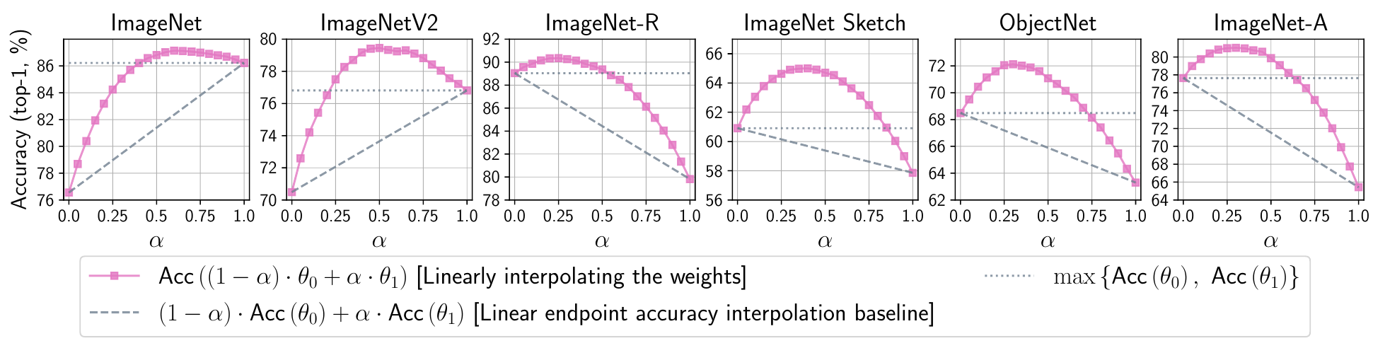
The pink curves rise in the middle. Every dataset has an interval that exceeds both endpoints, but their optima differ. These curves show the tradeoff and remind us that the best single coefficient depends on the data we need to serve.
Return to the first difficulty: small hyperparameter changes can substantially alter performance on shifted data, with little sign of it on ImageNet.
WiSE-FT turns this into adjusting just one . Even when the fine-tuning learning rate produces poor robustness, the authors find that adjusting with WiSE-FT can recover a good tradeoff between ImageNet and shifted data; changing requires no retraining. In their experiments, only weight-averaging methods reach this best tradeoff curve: WiSE-FT or an exponential moving average over all training iterates.
is a useful starting point, and gives this note its “halfway” subtitle, but no derivation requires it to be optimal everywhere. The appendix compares a fixed half-and-half mixture with the best value for each setting. Across the combined average of ImageNet and the five shifted datasets, the gap is about 0 to 0.4 percentage points. If a validation set represents the deployment setting, sweep the coefficient along the interpolation line. Each candidate still requires forward evaluation; the saving is in repeated fine-tuning.
Where does complementarity arise?
The authors first analyze the two classifiers in the fixed-feature LC setting. Alongside prediction disagreement, they examine which classifier determines the ensemble's result when the two disagree. The fine-tuned classifier more often dominates on ImageNet, while the zero-shot classifier more often dominates on most shifted datasets, with ImageNetV2 the exception.
This relates to the scale of confidence scores. Using the gap between the highest and second-highest logits as the margin, the authors find larger margins for the fine-tuned model on the reference distribution and for the zero-shot model on shifted data. When the models specialize in different examples, weighted logits can preserve that complementarity. This is an experimental analysis of LC. End-to-end fine-tuning also changes representations, which the authors discuss through empirical observations of the error landscape.
The paper also makes substantial baseline comparisons. The authors sweep learning rates, training duration, early stopping, and regularization toward zero-shot weights. In the LC setting, they also compare distillation toward zero-shot outputs, label smoothing, , and weight decay. Some recover part of the robustness, but require retraining or choosing a regularization strength. WiSE-FT's practical appeal is that fine-tuning can be completed first, then the tradeoff adjusted through inexpensive weight interpolation.
Its scope is specific. The main results concern natural distribution shifts; adversarial attacks and arbitrary unseen distributions lie outside that evaluation. Weight interpolation requires compatible architectures and class semantics. If even the encoders differ, the comparison must move to output ensembling; this one-line weight average no longer applies.
Conclusion
WiSE-FT fits in a single formula. Finish fine-tuning, then walk halfway back.
In this paper's setting, zero-shot and fine-tuned CLIP share pretrained weights, and both classification heads start from the same zero-shot classifier. Experiments along the line confirm a useful intermediate region. For your own models, first keep the checkpoint from before fine-tuning, then trace that line using validation data. That is usually easier than guessing another round of regularization coefficients.
Six months later, the same group took another step. Could all those fine-tuned models from different hyperparameter settings, otherwise discarded, also be averaged together? That paper is called Model Soups.