Original paper
Git Re-Basin: Merging Models modulo Permutation Symmetries
- Publication
- ICLR 2023Conference
- First submitted to arXiv
- arXiv:2209.04836
Cite this paper · BibTeX
The citation identifies the linked source version. It cites the original paper and its authors.
@misc{modelmerginggitrebasin2022,
  title = {{Git Re-Basin: Merging Models modulo Permutation Symmetries}},
  author = {Samuel K. Ainsworth and Jonathan Hayase and Siddhartha Srinivasa},
  year = {2022},
  eprint = {2209.04836},
  archivePrefix = {arXiv},
  url = {https://arxiv.org/abs/2209.04836}
}
Units in a hidden layer have no fixed order. Swap units 3 and 7, and swap the corresponding input positions in the next layer, and the network computes exactly the same thing.
Hecht-Nielsen discussed this permutation symmetry in 1990. It gives the same function an enormous number of different weight representations. The paper counts them for several common architectures:
| Architecture | Hidden-unit permutations |
|---|---|
| Three-layer MLP, width 512 | |
| VGG16 | |
| ResNet50 | |
| Upper bound on atoms in the observable universe |
Compiled from the original Table 1.
It has long been known that linear interpolation between networks trained from different random initializations can encounter a high barrier. In 2021, Entezari and colleagues proposed a bold conjecture: after accounting for possible permutations, most solutions found by SGD could be linearly interpolated without a barrier. In other words, the loss landscape might contain just one basin modulo permutations.
Samuel Ainsworth, Jonathan Hayase, and Siddhartha Srinivasa at the University of Washington wanted to turn that conjecture into a practical tool. Given two independently trained models, could a permutation “move” one into the other's basin so they could be averaged directly?
Defining the problem
The paper follows Frankle and colleagues in measuring a loss barrier:
This is the largest loss along the line minus the mean endpoint loss. A value of 0 indicates no rise above that reference.
The goal is to find a function-preserving permutation that minimizes the barrier between and . At layer , a permutation matrix transforms model B's weights into
reorders the output units of layer , while changes the order in which this layer reads its inputs to follow the preceding layer's permutation.
Input and output positions carry semantics, so both ends stay fixed. Image RGB channels and classifier class order cannot be swapped arbitrarily just to bring weights closer. Only internal hidden dimensions can move, and their biases, normalization parameters, and branch connections must move together. The two paths of a residual addition need compatible permutations; layers cannot be shuffled independently without these constraints.
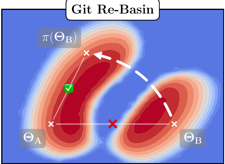
This schematic captures the paper's goal. and occupy different valleys, and their linear midpoint falls outside. Replacing with the functionally identical moves it into 's valley, with their midpoint inside as well.
Solving the problem
The authors propose three ways to find permutations.
Activation matching
The first is intuitive. Models solving the same task may learn similar features in different positions. Feed training data through both, collect layer activations , and find the permutation matrix that brings them closest:
The expression on the right is a classical linear assignment problem, solvable in polynomial time with algorithms such as the Hungarian algorithm. Each layer is solved independently, requiring just one pass through the data.
Weight matching
The second method uses no data at all, only weights.
Each row of the first layer's weights describes what a unit looks for. If row in A resembles row in B, those units may compute the same feature. Let's work through a small example with three units and four inputs:
import numpy as np
from scipy.optimize import linear_sum_assignment

# 模型 A 第一層的三個單元,各有 4 個輸入權重
W_A = np.array([[ 1.0, -0.5,  0.2,  0.0],
                [ 0.1,  0.9, -0.8,  0.3],
                [-0.6,  0.0,  0.4,  1.1]])

# 模型 B 學到差不多的三個單元,只是順序換成 (A 的第 2, 0, 1 個),數值也略有不同
W_B = np.array([[-0.5,  0.1,  0.5,  1.0],
                [ 0.9, -0.4,  0.1, -0.1],
                [ 0.2,  1.0, -0.7,  0.2]])

S = W_A @ W_B.T                       # S[i, j]:A 的單元 i 和 B 的單元 j 有多像
print(S.round(2))
rows, cols = linear_sum_assignment(S, maximize=True)
print("A 的單元 i 配到 B 的單元", cols)
[[-0.45  1.12 -0.44]
 [-0.06 -0.38  1.54]
 [ 1.6  -0.61 -0.18]]
A 的單元 i 配到 B 的單元 [1 2 0]
The maximum in each similarity-matrix row happens to identify the correct match. A's unit 0 matches B's unit 1, unit 1 matches unit 2, and unit 2 matches unit 0. The answer is visible at a glance here. Real networks have hundreds of units and less distinct similarities, so an assignment algorithm finds the pairing with the largest total score.
After finding a permutation, we still need to apply it correctly. Add an output layer and check model B's outputs before and after reordering:
W_out = np.array([[1., -2., 0.5], [0.3, 0.4, -0.7]])
x = np.array([0.2, -0.1, 0.5, 1.0])
before = W_out @ np.maximum(W_B @ x, 0)
W_B_aligned = W_B[cols, :]       # 隱藏層換列
W_out_aligned = W_out[:, cols]  # 下一層的輸入換欄
after = W_out_aligned @ np.maximum(W_B_aligned @ x, 0)
print("換位前後功能相同:", np.allclose(before, after))
換位前後功能相同: True
No models have been averaged yet; B has only been rewritten equivalently. Alignment itself should preserve B's output. Averaging it with A afterward changes the network's function. Checking these separately distinguishes an incorrectly applied permutation from a poor average.
The difficulty is that layers affect one another. A hidden unit's identity depends on both its incoming weights and the weights it sends to the next layer. Changing layer 's permutation also changes layer 's input order. Across all layers, the objective is
The authors prove that this “sum of bilinear assignments” is NP-hard; for three or more layers, even a constant-factor approximation has no polynomial-time solution under the stated hardness result.
Their compromise is coordinate descent. Fix every other layer and optimize only , reducing the problem to an ordinary linear assignment:
The first term compares incoming weights, already aligned to the preceding layer. The second compares outgoing weights, aligned to the following layer. Update layers in random order until permutations stop changing. The authors report convergence in seconds to minutes in practice.
Each accepted permutation increases the overall inner product, and there are finitely many permutations, so the procedure terminates. But its objective brings weights closer rather than directly minimizing data loss, and termination only identifies a point with no improvement available through these coordinate updates. In an ImageNet comparison restricted to one sweep, the merged model reaches only about 7% top-1 accuracy; repeated sweeps to convergence reach 51.01%. Aligning a layer once and never revisiting it misses information from subsequent layers.
Learning permutations with a straight-through estimator
The third method treats the permutation as learnable, minimizing the loss of the average of and the projected . Projection onto the nearest permutation is nondifferentiable, so it uses a straight-through estimator: the forward pass uses projected weights, while the backward pass treats projection as if it had not occurred.
This method performs best but requires an entire training loop, making it much more expensive.
More precisely, the optimizer maintains a freely adjustable . On each forward pass, it finds the closest among all equivalent permutations of B, then evaluates the training loss of . Projection still uses weight matching. During backpropagation, projection is approximated by the identity so gradients can reach . The final output is a permutation of the original B, so the B endpoint's function remains unchanged.
| Alignment method | Uses data? | Objective | Main cost |
|---|---|---|---|
| Activation matching | Yes, to collect intermediate representations | Match activations at each layer | Data forward pass and layer assignments |
| Weight matching | No | Whole-network weight inner product | Repeated layer assignment problems |
| STE matching | Yes, to compute merged loss | Midpoint training loss | Training loop and repeated projection |
With shared data and compatible architectures, activation matching or STE are options. When original training data are unavailable, weight matching still works. This least expensive choice is also the tool used later to merge separately trained models.
Discussion
Once aligned, the straight path opens

The datasets and models become more challenging from left to right. Direct interpolation, shown in gray, has a mountain in the middle of every plot. All three permutation methods lower it.
On MNIST, all three achieve zero barrier. Weight matching and STE even make the test-loss curve convex, with intermediate models outperforming both A and B. On CIFAR-10, widening ResNet20 by 32 times also achieves zero barrier, which the authors describe as the first such result on a ResNet to their knowledge. ImageNet's ResNet50 retains a small hill: the barrier is reduced by 67% relative to direct interpolation, but remains above zero.
The three methods differ relatively little. STE is best but most expensive. Weight matching needs no data and takes only seconds, yet performs similarly to data-dependent activation matching. The authors see it as a good balance of cost and effectiveness.
Some easily missed architectural details matter. The MLP has three hidden layers of 512 units each, ReLU, and no normalization. The CIFAR VGG and ResNet20 use LayerNorm, with cropping, rotation, and flipping, and are trained with momentum SGD. Only ImageNet's ResNet50 retains standard BatchNorm, with BatchNorm statistics recomputed for every interpolated model. Applying the method directly to standard BatchNorm-based CIFAR models may yield different curves.
The 67% figure is a relative reduction in the loss barrier, a different quantity from a 67-percentage-point accuracy gain. The ImageNet midpoint's 51.01% top-1 accuracy also shows that, after a large barrier reduction, the intermediate model can still be much weaker than either endpoint. The main achievement identifies conditions for low-barrier permutations; lossless merging of independent ImageNet models remains unresolved.
Wider networks connect more easily
Why does the ImageNet barrier remain? The authors suspect insufficient width.
They progressively widen VGG-16 and ResNet20 on CIFAR-10 and apply weight matching. Standard-width models do not show linear connectivity, but widening reduces the barrier all the way to 0. Their hypothesis is that a model needs enough capacity, especially width, to accommodate the data's complexity before linear connectivity emerges.
For narrow models, either the found permutation is inadequate or other symmetries, such as scaling across layers, remain unaccounted for. The discussion positions permutation symmetry as a “necessary but incomplete” part of the picture.
Learned during training
Another observation is that linear connectivity develops gradually during training. For MNIST and CIFAR-10 MLPs, the authors match and measure barriers after every epoch. Barriers are high early on and decline over training.
They also construct a counterexample: some solutions not found by SGD cannot connect linearly to other solutions under any permutation. This falls outside Entezari's conjecture, which concerns SGD solutions specifically, and suggests that SGD's own biases contribute to linear connectivity.
The counterexample has just two input dimensions and two hidden layers of two units each. Both models solve the same classification problem perfectly, but assign the decisions about the first and second dimensions to different layers. Within-layer permutations cannot transfer that division of work across layers. Every permutation of the small network can be enumerated, and the authors find a remaining barrier in every case. This is stronger evidence than simply failing to find a permutation, and illustrates that useful symmetries extend beyond unit reordering.
Train separately, merge together
The final experiment comes closest to a practical use. The authors split CIFAR-100 into two equal, disjoint datasets. Dataset A contains 20% of the examples from classes 0–49 and 80% from classes 50–99; dataset B reverses those proportions. They train one ResNet20 on each.
After weight matching and merging, the combined model has lower loss than either A or B on the full test set, uses half the memory and computation of an ensemble, and has better probability calibration than either original model. It still trails both a model trained on all the data and the two-model ensemble; direct interpolation performs much worse.
The two training sets are disjoint, but both models see all 100 classes, in opposite proportions. Their classification heads therefore retain consistent output semantics. Cross-entropy and calibration improve; classification accuracy does not exceed both original models. Describing the result simply as “train on different data, then merge for improvements across the board” would erase this tradeoff.
The appendix also considers multiple models. It repeatedly aligns one model to the average of all others, cycling through models before taking the overall average. Merging 32 MLPs, each seeing half of MNIST, gives calibration close to output ensembling while retaining one model at inference. This extends the demonstration beyond two models, though its scale and data complexity remain far from modern large language models.
Conclusion
Git Re-Basin turns the difficulty of averaging models from different initializations into a procedure: put the units in their seats, then average. Weight matching needs no data and can finish in seconds, reducing the barrier to zero in sufficiently wide networks.
It also marks the boundaries. Networks need enough width, and standard ImageNet ResNet50 still retains a barrier. Later, REPAIR finds that activation variance collapses in the averaged model after alignment; rescaling reduces ImageNet barriers further.
Many later large language model merges start with fine-tuned versions of the same pretrained checkpoint, using their shared parameter coordinates. Independently trained models first need the alignment problem addressed here, followed by checks of how much functionality survives the merge.