Original paper
Model Merging in LLMs, MLLMs, and Beyond: Methods, Theories, Applications and Opportunities
- Publication
- ACM Computing Surveys 2026Journal
- First submitted to arXiv
- arXiv:2408.07666
Cite this paper · BibTeX
The citation identifies the linked source version. It cites the original paper and its authors.
@misc{modelmergingmodelmergingsurvey2024,
  title = {{Model Merging in LLMs, MLLMs, and Beyond: Methods, Theories, Applications and Opportunities}},
  author = {Enneng Yang and Li Shen and Guibing Guo and Xingwei Wang and Xiaochun Cao and Jie Zhang and Dacheng Tao},
  year = {2024},
  eprint = {2408.07666},
  archivePrefix = {arXiv},
  url = {https://arxiv.org/abs/2408.07666}
}
Papers on model merging have multiplied quickly over the past few years, and so have the names.
Task arithmetic, TIES, DARE, AdaMerging, RegMean, Fisher Merging, Model Breadcrumbs, TSV-M, WEMoE... Every paper says it solves some kind of interference in merging, but few people have looked at them side by side and asked which problem each method actually addresses, what data it needs, and whether it still holds up on large language models.
This survey by Yang, Shen, Guo and colleagues at Sun Yat-sen University (Shenzhen Campus), Northeastern University and Nanyang Technological University sets out to answer those questions. It was first released in August 2024 and has been updated continually since; the fifth version, from late 2025, has grown to forty pages. The authors also maintain a GitHub paper list that keeps adding new work.
This note focuses on its taxonomy, the comparison experiments the authors ran themselves, and the problems it considers still unsolved.
Defining the problem
How model merging differs from other approaches
The authors begin by comparing model merging with four related ways of learning.
- Single-task learning: train one expert model per task. The tasks do not interfere with one another, but knowledge cannot be shared, and the number of models grows with the number of tasks.
- Multi-task learning: one model learns all tasks at once, but training needs the data for every task together.
- Federated learning: the data stays with each client and a server aggregates model updates, but many communication rounds are needed.
- Ensemble learning: keep several expert models at once and combine their outputs, which makes both inference and storage expensive.
Model merging instead combines the parameters of several trained expert models directly into a single model, and in most cases it needs neither the original data nor further training.
Formally, given models with the same architecture, , usually fine-tuned from the same pretrained model , the goal is to find
The simplest version is plain averaging. The authors point out that averaging often works poorly, for two kinds of reasons. One is that the prerequisites for merging are missing, for example the models do not sit in the same basin or their architectures differ. The other is that the parameters for different tasks conflict and interfere with one another.
The survey's entire taxonomy of methods is organized around these two causes.
Solving the problem
Taxonomy: before merging and during merging
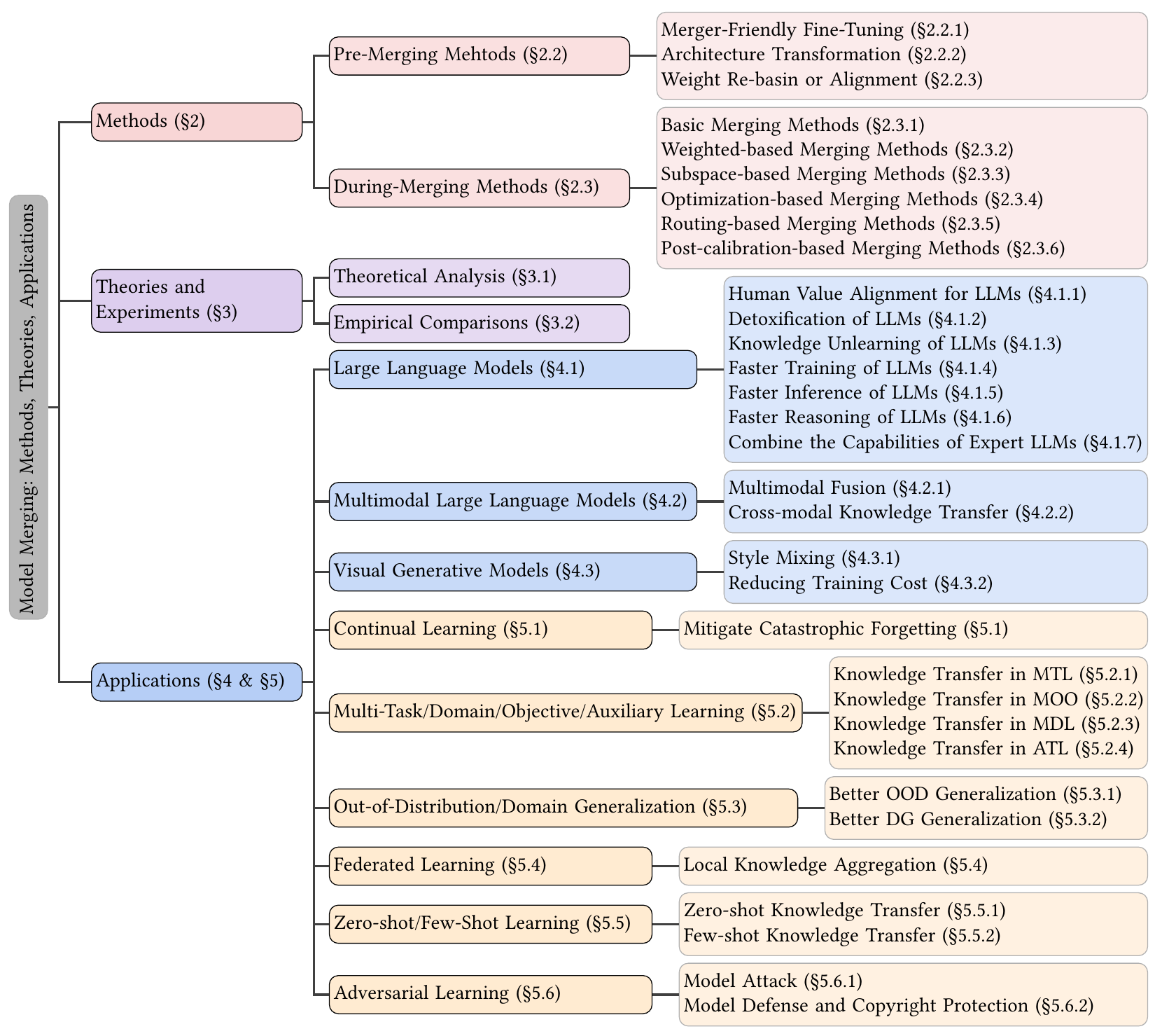
This figure is the table of contents for the whole survey. The “Methods” branch at the top splits into two points in time.
Pre-merging methods aim to create good conditions for merging:
- Merger-friendly fine-tuning: make models easier to merge while they are still being fine-tuned. The representative work is task arithmetic in the tangent space, which fine-tunes a linearized model so that task vectors are more disentangled. Follow-up work linearizes only some layers to cut the cost, or uses sharpness-aware minimization to make the loss landscape flatter, and other approaches fine-tune only a small fraction of the parameters to reduce conflicts.
- Architecture transformation: models with different architectures cannot have their parameters merged directly, so knowledge distillation or added layers first turn them into the same architecture. FuseLLM and FusionChat belong here, at the cost of needing data and training.
- Weight re-alignment: independently trained models first go through neuron permutation alignment so that they land in the same basin. Git Re-Basin and the optimal-transport alignment method OTFusion belong here. The authors also cite REPAIR's observation that how well alignment works depends heavily on the normalization layers.
During-merging methods handle conflicts between tasks and fall into six categories:
- Basic methods: plain averaging, or task arithmetic.
- Weighted methods: decide weights for different models, different layers or even individual parameters. Examples include searching coefficients with evolutionary algorithms, AdaMerging learning coefficients on unlabeled test data with entropy as a proxy loss, RegMean solving a closed form for linear layers, and Fisher Merging measuring parameter importance with Fisher information. SLERP is also placed in this category.
- Subspace methods: project task vectors into sparse or low-rank subspaces. Sparse methods include TIES-Merging, DARE and Model Breadcrumbs; low-rank methods include TSV-M, ISO-C and KnOTS, which apply SVD to task vectors.
- Optimization methods: use properties of the task vectors themselves to write objective functions that need no data, for example making task vectors more orthogonal (AWD) or building a data-free loss on linear layers (WUDI-Merging).
- Routing methods: the categories above all produce one fixed model, whereas routing methods decide how to merge dynamically, depending on the input. WEMoE, for example, merges linear layers with weights from a routing network. These methods usually perform best, at the cost of keeping extra parameters and slower inference.
- Post-calibration: the internal representations of a merged model differ substantially from those of each expert. Methods such as Representation Surgery add a small module that corrects this bias.
What a comparison table shows
The authors lay out representative methods along several dimensions: parameter count after merging, whether the method needs tuning, what data it requires, whether it is static or dynamic, and the granularity of its weights (global, task, layer or parameter). Set side by side, several tradeoffs become obvious.
- The vast majority of methods end up with one model's worth of parameters. Routing and calibration methods exceed one model, and WEMoE far exceeds it.
- Finer-grained weighted methods usually perform better, but most of them need extra data, such as a validation set or an unlabeled test set, to estimate the weights.
- Many optimization and low-rank subspace methods advertise that they need no data.
The authors conclude that no single method suits every situation; the choice depends on performance requirements, implementation difficulty, and the data and compute at hand.
Theory is still fragmented
Section 3 surveys theoretical analysis and divides it into three categories by where the merged models come from.
- The same training trajectory: for methods such as SWA and EMA, in simplified settings such as least-squares regression, there are bias–variance decompositions as well as stability and generalization bounds for both convex and nonconvex cases.
- The same task, different hyperparameters: explained through linear mode connectivity and flat minima. Models fine-tuned from the same pretrained model with different settings are usually linearly connected.
- Different tasks: task arithmetic is explained through the NTK and weight disentanglement. Some studies also link task vectors to gradients; when training for one epoch with full-batch gradient descent, the task vector is exactly the learning rate times the negative gradient.
The authors admit that these three lines of theory each cover only part of the picture. Most rest on assumptions of a shared starting point, wide networks or linearization; whether they carry over to large language models has not been verified, and there is still no unified framework.
Discussion
The authors' own comparison
The survey also includes a set of comparison experiments the authors ran themselves, covering five backbones: CLIP's ViT-B/32 and ViT-L/14 merging 8 image classification tasks, RoBERTa-Large merging 8 GLUE tasks, Llama-3.1-8B merging 5 text generation tasks, and InternVL-2.5 merging 5 multimodal tasks.
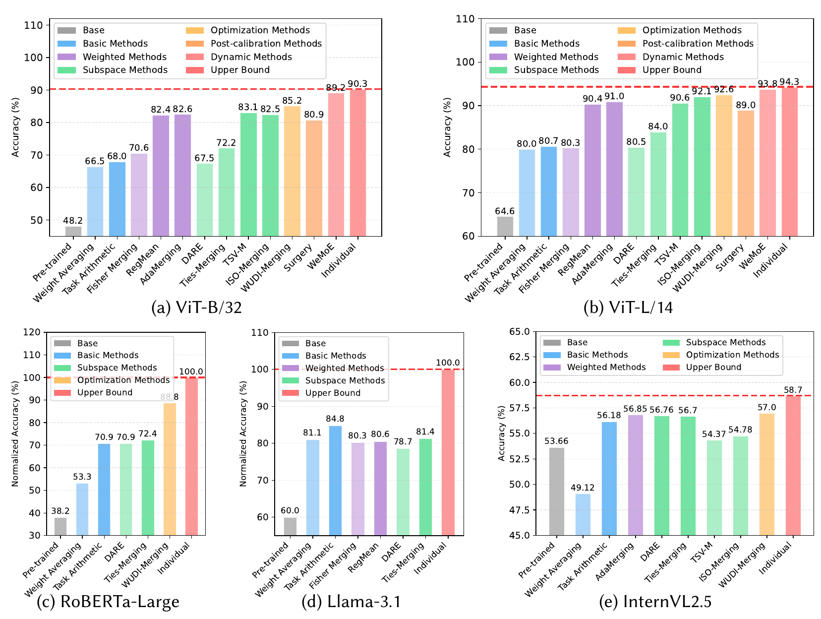
In each chart, the gray bar on the far left is the pretrained model, and the red bar on the far right is the model fine-tuned separately for each task, which is the upper bound. For the methods in various colors in between, the closer to the red dashed line, the better.
Start with ViT-B/32. Plain averaging reaches only 66.5, far below the upper bound of 90.3. Weighted and low-rank subspace methods pull it up to 82–83, data-free WUDI-Merging reaches 85.2, and the routing method WEMoE, which needs extra parameters, reaches 89.2, nearly matching the upper bound. On ViT-L/14 every method does much better, with WEMoE at 93.8 against an upper bound of 94.3. Larger models are easier to merge, in line with the observation in Bigger is easier to merge.
Llama-3.1 is a very different story. Task arithmetic comes first at 84.8. Fisher Merging, RegMean, DARE and TIES all land between 78.7 and 81.4, below task arithmetic and only slightly above or below plain averaging at 81.1, and the gap to the upper bound of 100 is still more than ten points. The “advanced” methods that clearly win on vision tasks show no advantage on the generation tasks of a language model.
On InternVL2.5, plain averaging scores 49.12, even below the pretrained model's 53.66, so merging actually makes the model worse. The methods differ by only a point or two; the best, WUDI-Merging, reaches 57.0 against an upper bound of 58.7.
This comparison is one of the most valuable parts of the survey. Many merging methods were developed and tuned on CLIP's eight classification tasks, and the rankings get reshuffled once you move to LLMs and multimodal models. Before picking a method, it is best to rerun the comparison on your own model and tasks.
Seven uses in large language models
Section 4 lists applications of model merging to LLMs, and several of them connect to other notes on this site.
- Aligning with human preferences: train models that fit different preferences separately, then merge them according to what each user needs.
- Detoxification: remove toxic or untruthful outputs by subtracting task vectors.
- Unlearning: use the same kind of subtraction to remove specific knowledge, such as copyrighted material learned by mistake, without paying to retrain from scratch.
- Faster training: average checkpoints during pretraining. The authors file both PMA and WSM here; both treat checkpoint averaging as a substitute for learning-rate decay.
- Faster MoE inference: merge expert parameters before computing, so that fewer experts need to be evaluated.
- Faster reasoning: merge a reasoning model that thinks at length with a general model that answers briefly, to shorten the output. In the examples the authors cite, task arithmetic and TIES cut reasoning length by about half on 7B models, with accuracy roughly unchanged.
- Combining expert capabilities: merge expert models from different domains into a single general-purpose model.
As for how merging is actually used in technical reports, the survey says little. For the details of how reports such as Llama 3, Tülu 3 and Command A write merging into their official training pipelines, you have to go back to each report.
Open problems
The final section lists seven directions, and the first few are the most practical.
- The gap to independent models: merging still depends heavily on the premise of “the same pretrained model, with the fine-tuning learning rate and number of steps carefully controlled.” Even then, the gap becomes obvious as the number of tasks grows; on Llama-3.1, for example, the best method scores 84.8 against an upper bound of 100.
- Theory: there is almost no theoretical explanation for merging models trained from scratch on different tasks.
- Trustworthiness: model owners want to protect their models from being merged, while those doing the merging need to guard against backdoors hidden in models.
- Efficiency: high-performing methods usually need every model loaded into memory at the same time; merging 72 fine-tuned ViT-B/32 models, for instance, takes more than 200GB. Searching for coefficients also requires repeated evaluation.
- Heterogeneous models: models with different architectures currently have to be distilled into a common architecture first, which is expensive.
How to read this survey
This is a very broad survey. Section 5 also takes in more than ten subfields, including continual learning, multi-task learning, out-of-distribution generalization, federated learning, few-shot learning and adversarial attacks, usually giving each only a paragraph or two.
So what is it best used for? Its taxonomy works as a map. When you meet a new merging method, work out whether it is a pre-merging or during-merging method, what data it needs and whether it is static or dynamic, and you will roughly know which problem it addresses and what it costs. For the details of a specific method and its experimental conditions, you still have to check the original paper.
Conclusion
Using two stages, “pre-merging” and “during-merging,” this survey organizes scattered merging methods into one clear map, and fills in theory, applications and open challenges.
The most valuable takeaway is the authors' own comparison. Advanced methods that perform well on CLIP do not necessarily beat the simplest task arithmetic on Llama-3.1.
With this many methods around, use task arithmetic as the baseline first and take it from there.