Original paper
Model Merging in Pre-training of Large Language Models
- Publication
- NeurIPS 2025Conference
- First submitted to arXiv
- arXiv:2505.12082
Cite this paper · BibTeX
The citation identifies the linked source version. It cites the original paper and its authors.
@misc{modelmergingpretrainingmerging2025,
  title = {{Model Merging in Pre-training of Large Language Models}},
  author = {Yunshui Li and Yiyuan Ma and Shen Yan and Chaoyi Zhang and Jing Liu and Jianqiao Lu and Ziwen Xu and Mengzhao Chen and Minrui Wang and Shiyi Zhan and Jin Ma and Xunhao Lai and Deyi Liu and Yao Luo and Xingyan Bin and Hongbin Ren and Mingji Han and Wenhao Hao and Bairen Yi and LingJun Liu and Bole Ma and Xiaoying Jia and Xun Zhou and Siyuan Qiao and Liang Xiang and Yonghui Wu},
  year = {2025},
  eprint = {2505.12082},
  archivePrefix = {arXiv},
  url = {https://arxiv.org/abs/2505.12082}
}
The hardest part of pretraining a large language model is not knowing how good it will turn out.
The learning-rate schedule in common use today is called WSD (Warmup-Stable-Decay). It warms up briefly, trains at a constant learning rate for a long stretch, and finally lowers the learning rate to “anneal.” The trouble is that checkpoints from the constant-learning-rate phase always score low, and the model's final level only shows after annealing. To find out whether training is heading in the right direction, you have to split off a separate branch and anneal it, at a cost of tens of billions to more than a hundred billion extra tokens every time.
Most model merging research happens after fine-tuning, combining several models trained for different tasks. Merging during pretraining is a different matter, combining checkpoints along a single training trajectory. The technical reports of Llama 3 and DeepSeek-V3 both mention using this kind of technique without giving details, and ordinary researchers cannot get hold of intermediate checkpoints from large-scale pretraining, which makes the topic hard to study on their own.
This paper from ByteDance Seed trains a series of dense and MoE models from scratch, up to 200B total parameters, and measures checkpoint merging during pretraining in detail. The authors call the approach PMA (Pre-trained Model Average).
Defining the problem
What gets merged are checkpoints saved in sequence along one training trajectory, and the merged model is their weighted sum:
Adjacent checkpoints are separated by a fixed amount of training , counted in tokens. For example, and means taking the 10 checkpoints saved every 8B tokens within the most recent 80B tokens.
For the weights , the paper compares three common schemes:
- SMA (simple moving average): every checkpoint weighs the same, .
- EMA (exponential moving average): computed recursively as , so newer checkpoints get more weight; the larger is, the more it favors the latest checkpoint.
- WMA (weighted moving average): weights grow linearly, for example , and are then normalized by their sum.
With , for example, the SMA weights are and the WMA weights are .
The authors break the study into six questions: how merging affects performance, which merging method works better, how to choose the interval and the number of checkpoints, whether the merged model helps as the starting point for the next stage, whether merging can improve training stability, and why merging works.
The experiments use an internal corpus and internal architectures. MoE models range from 0.7B/7B (active/total parameters) to 20B/200B, and dense models from 411M to 70B. Evaluation covers sixteen public benchmarks, including MMLU, BBH, GSM8K and HumanEval, and most figures report their weighted average score.
Solving the problem
Constant learning rate: plain averaging already helps
The first experiment is the simplest. After training for a while in the constant-learning-rate phase, the authors average the checkpoints and compare the result with the latest checkpoint.
MoE models of all four sizes improve clearly. Seed-MoE-1.3B/13B's HumanEval rises from 31.1 to 36.6, and Seed-MoE-10B/100B's from 54.3 to 61.6. Larger models gain less on nearly saturated benchmarks such as BBH. The dense models in the appendix show the same thing, with Seed-Dense-70B's HumanEval rising from 50.6 to 57.9 and GSM8K from 85.9 to 91.3, and the gains do not shrink as the models get larger.
This is the same intuition as SWA from 2018. When the learning rate is constant and fairly large, the model bounces back and forth near the valley floor, and each checkpoint stops at a different spot on the valley walls. Averaging them lands closer to the center of the valley.
Annealing: an early average catches up with the finish
The second experiment merges during the annealing phase. The learning rate decreases along a cosine curve, and the model's scores keep climbing.
Interestingly, merging checkpoints right at the start of annealing already gives scores about as good as those at the end of annealing; larger models sometimes even beat the result of annealing all the way through.
That raises a bolder question. If merging can achieve what annealing does, can we skip annealing altogether?
Merging without annealing
The authors branch Seed-MoE-1.3B/13B at 1.4T tokens into two runs. One keeps the constant learning rate and the other starts annealing, and each trains for another 250B tokens. They then merge checkpoints from the constant-learning-rate run.
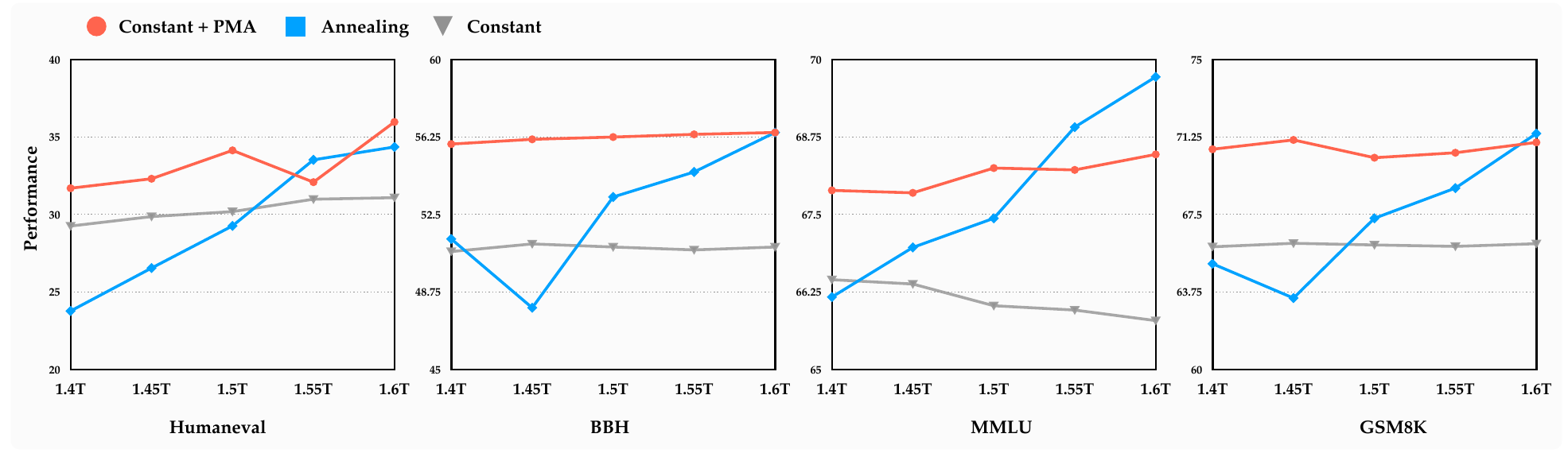
Look at the gray and red lines first. Both use a constant learning rate. The gray line without merging barely improves, and on MMLU it even keeps sliding, while the merged red line starts a notch higher.
Then the blue line. Scores early in annealing are usually lower, and on BBH and MMLU they even dip before climbing steadily. By 1.6T, the red and blue lines are about even on HumanEval, BBH and GSM8K, while on MMLU annealing comes out clearly higher, by about two points.
The authors conclude that a constant learning rate plus merging can roughly predict post-annealing performance at any point in training, which makes it a cost-effective tool for quick validation. The conclusion holds on three benchmarks; MMLU is an exception worth remembering when reading the figure.
How to merge: method, interval and count
Method. On Seed-MoE-1.3B/13B at 204B training tokens, all three methods beat the unmerged model. WMA is best, and EMA with also beats . Early in training the weights change a lot, so newer checkpoints deserve more weight. Later in training, the differences between the three methods almost disappear. From here on, the authors use the simplest one, SMA.
Interval . With fixed, they compare values of 4B, 8B, 16B and 32B tokens. Early in training (204B tokens), intervals of 16B and 32B are actually worse than not merging, because reaching that far back mixes in weights from the start of training, when they were still very unstable. The longer training runs, the smaller the differences between intervals.
The authors derive a rule of thumb that scales with model size: about 4B tokens for 0.7B/7B models, 8B for 1.3B/13B, and 80B for 10B/100B. Larger models usually train with larger batches, so the interval between checkpoints stretches along with them.
Count . With fixed, they compare 3, 6, 10 and 15 checkpoints. Taking too many early in training again mixes in unstable weights; later in training, more is better, and scores nearly 1 point higher than . The authors settle on as a compromise.
The merged model as the next stage's starting point
Pretraining is usually followed by continued training (CT), SFT and reinforcement learning. The authors use the merged weights as the starting point for the next stage and call this PMA-init.
CT stage. On Seed-MoE-0.7B/7B, they merge after training on about 1T tokens and then continue with CT. PMA-init starts with a slightly lower loss and is also better on MMLU early on, but later in training the two losses converge to about the same level and the overall scores are even. Several different learning-rate schedules all lead to the same conclusion.
SFT stage. On Seed-MoE-15B/150B, they run 220M tokens of SFT starting from the merged weights. At the same learning rate, PMA-init moves MMLU from 86.8 to 87.1, LiveBench from 50.5 to 52.0 and AMC-2023 from 61.0 to 64.0, and the internal OOD and instruction-following evaluations each gain more than two points.
The authors also honestly report that gains of this size could not be reproduced at other model sizes. PMA-init does not hurt downstream performance and sometimes helps, with no guarantee that it helps every time.
Rescuing loss spikes
PMA-init has another, more unexpected use.
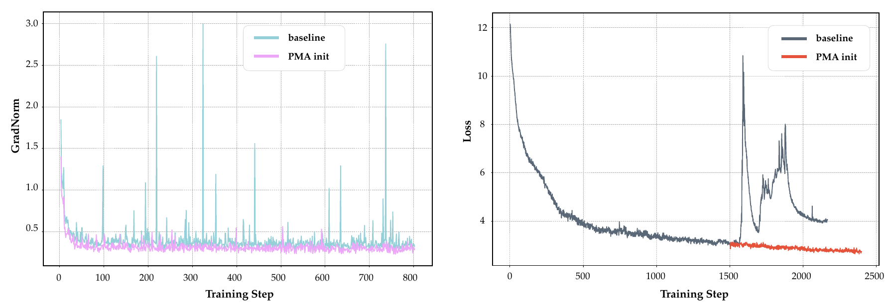
The left plot shows the gradient norm during SFT. The PMA-init curve is clearly steadier, with fewer loss spikes as well.
The right plot is an unstable training run the authors created on purpose. Studying loss spikes directly on large models is too expensive, so they use a small 330M/3.3B MoE model with an unusually large learning rate of 6e-3 to reproduce the kind of spike common in large models. After the spike, the original run never gets back to its original trajectory. The authors merge three checkpoints saved before the spike and restart from there, and training passes steadily through the point where things had gone wrong.
This gives large-scale training a practical option. When a run cannot recover from a loss spike, you do not have to roll back to a much earlier checkpoint or start over. Average the few checkpoints from just before the spike and continue training from there.
Discussion
Why averaging does better
The authors explain this with a second-order expansion of the loss around the optimum . Let each checkpoint's deviation from the optimum be and the Hessian be ; the gradient is zero at the optimum, so
The averaged model's deviation is . Expanding both sides and comparing them, the merged model's loss is lower than the average loss of the individual models when
When is positive definite, the right-hand side is always positive. If the cross terms on the left are mostly negative, meaning the checkpoints deviate from the optimum in “complementary” directions, the condition is easily met.
Try the most extreme cases with two checkpoints. If , the two points sit on opposite sides of the optimum, and their average lands exactly on , at the lowest loss . If , the two points coincide and averaging brings no benefit at all.
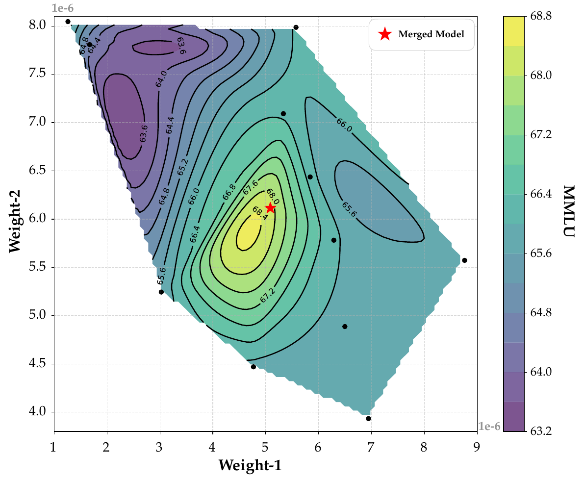
The authors also pick two parameters from one layer of Seed-MoE-1.3B/13B and plot them. The checkpoints are scattered around the high-score region, and the averaged red star sits closer to its center.
This also explains why merging checkpoints after annealing has limited effect. Once the learning rate is very low, the checkpoints are all crowded into the same small valley floor. Their deviations no longer point in complementary directions, so averaging has nowhere better to go.
This analysis does rest on quite a few assumptions, though. It assumes that the checkpoints all lie near the same optimum, that the second-order approximation holds and that the Hessian is positive definite; in nonconvex pretraining, all of these are only approximations. The two-parameter contour plot is a tiny slice of an extremely high-dimensional space, and the authors themselves use it only to build intuition.
Things to keep in mind when reading this paper
All the models, architectures and corpora are internal and cannot be reproduced. The main metric is a weighted average of sixteen benchmarks, and the weights are not published. The rule of thumb for intervals comes from MoE models of three sizes; with different batch sizes or data mixtures, the numbers may not carry over.
On the other hand, experiments at this scale are rare in the public literature. The ablations span from a few hundred million parameters to two hundred billion total parameters, which makes the paper a very concrete reference for any team that wants to add checkpoint averaging to its own pretraining pipeline.
A few months later, WSM went further in the same direction, replacing learning-rate decay entirely with checkpoint merging.
Conclusion
This paper turns “averaging checkpoints during pretraining” from a single sentence in technical reports into experimental results backed by systematic ablations.
Averaging the most recent checkpoints in the constant-learning-rate phase raises scores noticeably and roughly predicts post-annealing performance. SMA is good enough, the interval should grow with model size, and more checkpoints help later in training. PMA-init does no harm in CT and SFT, and it can pull a run with an otherwise unrecoverable loss spike back on track.
If you want to peek at the results halfway through pretraining, you can average the last ten checkpoints first. The hundreds of billions of tokens that annealing costs can wait.