Original paper
REPAIR: REnormalizing Permuted Activations for Interpolation Repair
- Publication
- ICLR 2023Conference
- First submitted to arXiv
- arXiv:2211.08403
Cite this paper · BibTeX
The citation identifies the linked source version. It cites the original paper and its authors.
@misc{modelmergingrepair2022,
  title = {{REPAIR: REnormalizing Permuted Activations for Interpolation Repair}},
  author = {Keller Jordan and Hanie Sedghi and Olga Saukh and Rahim Entezari and Behnam Neyshabur},
  year = {2022},
  eprint = {2211.08403},
  archivePrefix = {arXiv},
  url = {https://arxiv.org/abs/2211.08403}
}
By late 2022, the literature held two contradictory results on whether two networks can be averaged directly once their permutations are aligned.
On one side, Singh and Jaggi aligned neurons with optimal transport in 2020. For two ResNet18s with over 93% accuracy on CIFAR-10, linear interpolation after alignment gave a midpoint of 77% at best, still 16 percentage points short.
On the other side was Git Re-Basin from September 2022. On widened ResNets, it brought two independently trained CIFAR-10 models to nearly zero barrier. One of the alignment methods it compared, “activation matching,” is precisely a special case covered by Singh and Jaggi's method.
How could both results hold at the same time?
This paper, written by Keller Jordan of Hive AI together with Sedghi, Saukh, Entezari and Neyshabur of Google and TU Graz, supplies the answer. The last four are the same group that proposed the permutation invariance conjecture.
Defining the problem
The survey by Entezari et al. in the previous paper had already shown that the barrier after alignment falls with width but rises sharply with depth. For MLPs or CNNs more than a few layers deep, even alignment cannot save them.
The authors wanted to know what exactly depth breaks.
Instead of further refining alignment algorithms, they opened up the interpolated network and looked at the activations of each layer. The measurement is simple. For a given layer, compute each neuron's activation variance over a batch of training data and sum these into . Then compare the interpolated model's with the endpoint models' and :
A ratio near 1 means the interpolated model's activations are as active as the endpoint models'; a ratio near 0 means the layer's output barely changes with the input.
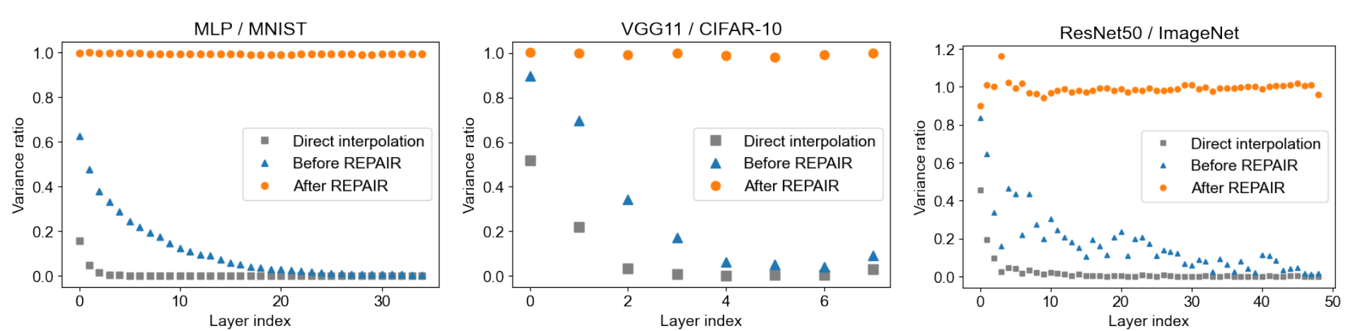
Look at the blue triangles first, which show the interpolated model after alignment and before any correction. The MLP's first-layer variance ratio is about 0.6. From there it falls layer by layer and is almost zero in the last few of its 35 layers. VGG11 and ResNet50 behave the same way, with the variance in their last few layers down by more than a factor of ten.
The authors call this phenomenon variance collapse. Activations in the last few layers are nearly constant, so the network can no longer tell different inputs apart, and accuracy naturally suffers.
The gray squares, direct interpolation without alignment, collapse even faster.
Solving the problem
Why the variance shrinks
Start with the first layer of the interpolated network. The input to the first layer is the raw data, so a neuron's preactivation after interpolation (its value before ReLU) is exactly a linear combination of the corresponding neurons at the two endpoints:
Treat and as random variables that vary with the data. At the midpoint ,
The first term is the variance we would hope for, namely the square of the averaged endpoint standard deviations. The second term is the part that gets subtracted, and it is subtracted whenever the correlation between the two neurons is below 1.
If the two endpoints have similar standard deviations, the expression simplifies to
However good the alignment, two independently trained networks will not learn exactly the same neurons. The authors observe that neurons paired up by alignment usually have a correlation of only about 0.4. Plugging that in,
the first layer loses 30% of its variance.
Deeper layers cannot be derived this precisely, because their inputs are already the shrunken activations of the previous layer. The authors' intuition is that the loss compounds from layer to layer. As a rough assumption, if each layer keeps only 70%, then after 10 layers only remains.
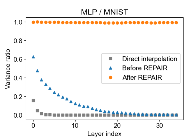
Compare this rough estimate with the MLP measurements. The blue triangles start at about 0.62 at layer 0, are still at about 0.12 at layer 10, and only fall to around 0.03 near layer 20. The actual decay is slower than 70% per layer, but the shape of a layer-after-layer decline is the same.
What REPAIR aims for
Since the problem lies in the statistics, fix the statistics. For each channel to be corrected, REPAIR requires the interpolated model to satisfy two conditions:
The condition on the mean already holds on its own; what actually breaks is the second one. Before correction, typically .
As for which channels to correct, the authors choose the output of every convolutional layer in VGG. For ResNet, they add the output of every residual block to the convolutional outputs.
The approximate version: one scaling factor
For the first layer alone, the correction factor can be computed directly. After measuring , and on the endpoint models, the variance of the interpolated neuron is
The required scaling factor is simply “the target standard deviation divided by the actual standard deviation”:
With the earlier numbers, and equal endpoint standard deviations, , so each neuron's output only needs to be scaled up by 20%.
This factor is exact for the first layer and only approximate for deeper ones. The authors test it on MLPs with 2 to 50 layers trained on MNIST. Without correction, the midpoint model drops below 90% once there are more than 6 layers; with this approximate correction, it stays above 90% all the way to 27 layers.
The advantage of the approximate version is that it needs forward passes only on the endpoint models. Once the statistics are computed, the correction factor for any follows directly.
The exact version: let BatchNorm do the measuring
The approximate version falls short on hard cases such as ResNet50 on ImageNet. The authors therefore propose an exact version that runs forward passes directly on the interpolated model.
The approach is to temporarily attach a BatchNorm layer after every module to be corrected:
from torch import nn

class RepairWrap(nn.Module):
    def __init__(self, module, channels):
        super().__init__()
        self.module = module
        self.bn = nn.BatchNorm2d(channels)      # newly added layer, starts in train mode

    def set_goal(self, goal_mean, goal_std):
        self.bn.bias.data = goal_mean            # (1-α)·E[X1] + α·E[X2]
        self.bn.weight.data = goal_std           # (1-α)·std(X1) + α·std(X2)

    def forward(self, x):
        return self.bn(self.module(x))
In training mode, BatchNorm first normalizes its input to mean 0 and variance 1, then multiplies by weight and adds bias. Set these two parameters to the target standard deviation and mean, and the output statistics come out exactly as the conditions require.
Next, about 5,000 training examples are fed through the network so that the new BatchNorm layers can estimate their running mean and running variance, while all of the network's original BatchNorm layers stay frozen. After estimation, the model switches to evaluation mode, and each new layer becomes a fixed scale and shift that can finally be fused into the weights of the preceding convolution, leaving the model architecture exactly as it was.
There is an interesting parallel here. If a network already has BatchNorm after every convolution, correcting only the convolution outputs is mathematically equivalent to re-estimating the BatchNorm statistics. SWA already treated averaged models this way in 2018, but no one had applied it between two independently trained networks. REPAIR extends the approach to residual block outputs and to networks without BatchNorm.
REPAIR complements alignment algorithms. Throughout the paper, the authors use the activation-correlation matching of Li et al. (2015), solved with the Hungarian algorithm. In networks with residual connections, all layers on the same residual stream must share the same permutation.
Discussion
ResNet18 on CIFAR-10
For two aligned ResNet18s, the endpoints score 95.5% on the CIFAR-10 test set. The midpoint of direct interpolation reaches only 66.0%; after REPAIR the midpoint is 94.1%, leaving a barrier of just 1.5 percentage points. For comparison, Singh and Jaggi's optimal-transport alignment has a midpoint of 77.0%.
Normalization layers resolve the contradiction
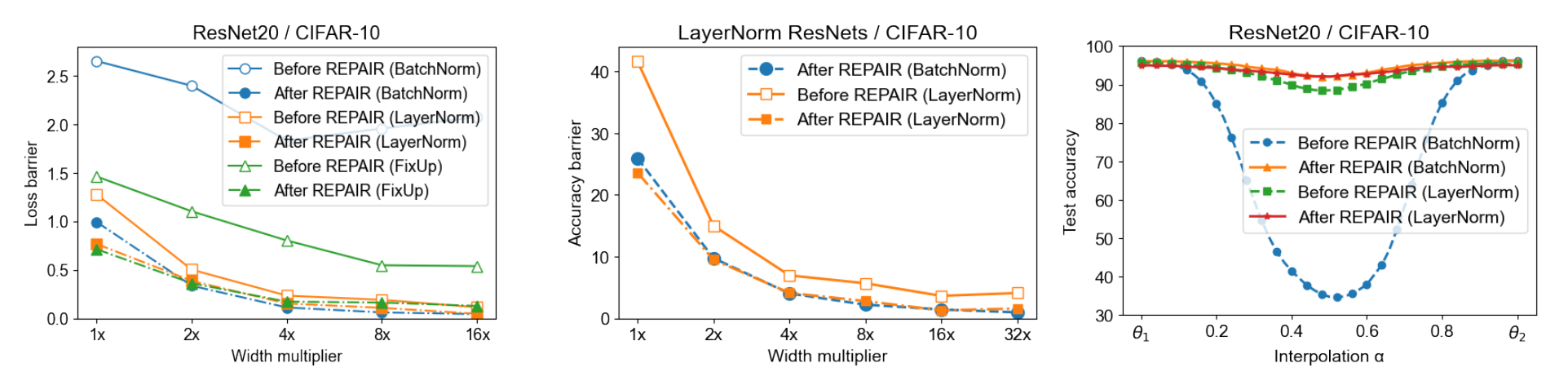
The authors train ResNet20 on CIFAR-10 and compare three normalization choices, BatchNorm, LayerNorm and Fixup without normalization, at width multipliers from 1× to 16× (the last block going from 64 to 1024 channels).
The right panel is the most convincing. Before correction, the standard-width BatchNorm version drops to 34.7% at the midpoint, while the LayerNorm version already has 88.4%. After correction, both reach 92.0%.
The same pattern holds at 8× width. The LayerNorm midpoint is already at 90.3% before correction and reaches 93.2% after; BatchNorm has only 32.3% before and 94.4% after. The left panel shows that at 16× width, the corrected loss barriers of both BatchNorm and LayerNorm are below 0.05.
Why is LayerNorm special? The authors' explanation is that LayerNorm renormalizes according to the current input even at inference, so the variance each layer loses gets pulled back rather than accumulating. At inference, BatchNorm is just a fixed affine transformation, so the shrinkage stacks up layer after layer.
That resolves the contradiction raised at the outset. The authors checked Git Re-Basin's code and found that its ResNets replace BatchNorm with LayerNorm. Singh and Jaggi used a standard BatchNorm ResNet18, so however good their alignment was, variance collapse dragged it down.
LayerNorm has a cost too. Under the same training setup, the LayerNorm ResNet20 reaches 92.4% on CIFAR-10, against 93.6% for the BatchNorm version.
ImageNet
On ImageNet, direct interpolation after alignment gives midpoint accuracy below 1% for ResNet18, ResNet50 and a double-width ResNet50. After REPAIR, they reach 41.1%, 56.5% and 64.2% respectively.
Whether to correct the residual block outputs makes a sizable difference. For ResNet50, correcting only the convolution outputs gives a midpoint of 53.2%; adding the residual block outputs raises it to 56.5%, and the barrier falls from 23.4 percentage points to 20.1.
That is still a large barrier, though. After correction, the standard ResNet50 is still left with 20.1 percentage points, and the double-width version with 12.9. The authors speculate that hard datasets need wider networks before the barrier gets very low.
Width and depth
For 10-layer MLPs (width 32 to 2048) and ResNet20 (width 1× to 16×), across the four datasets MNIST, FashionMNIST, SVHN and CIFAR-10, REPAIR lowers the barrier every time, and the wider the network, the lower it goes. On MNIST even the narrower networks get close to zero.
As for depth, for VGG on CIFAR-10 from 11 to 19 layers, the barrier rises with depth before correction and becomes almost independent of depth after correction. The “depth raises the barrier” pattern seen in Entezari et al.'s survey comes at least partly from variance collapse.
Merging models trained on different data
The last experiment reproduces Git Re-Basin's setup. The 50,000 CIFAR-100 training images are split into two sets of 25,000. The first set takes 80% of the first 50 classes and 20% of the last 50, and the second set the reverse. Each network is good at half of the classes.
After alignment and REPAIR, many models along the interpolation path have lower loss on the full test set than both endpoints. The best is at , with a test loss of 1.30; the best value Git Re-Basin reported was 1.73, also at . The authors candidly say that this gap comes partly from REPAIR and partly from the standard ResNet simply being stronger than the LayerNorm version.
Is this still a permutation?
In their discussion, the authors raise an honest question. REPAIR achieves low barriers in more cases, which seems to support Entezari's conjecture; but it rescales the preactivations of the interpolated model, so it is no longer strictly “linear interpolation after permutation.”
In other words, at practically usable widths and without switching to LayerNorm, permutation alone seems insufficient, and this kind of statistical correction is needed as well. The conjecture itself remains unproven.
In practice, remember also that REPAIR needs training data. The endpoint models' statistics are measured on training data, and the exact version feeds several thousand more examples through the interpolated model. If you have only the weights and no data, this step is out of reach.
Conclusion
This paper traced what looked like an alignment problem to the statistics inside the interpolated network. Unless two neurons are perfectly correlated, averaging shrinks the variance, and BatchNorm networks let that shrinkage compound layer after layer until the whole network stops responding to its input.
The fix simply pulls each channel's mean and standard deviation back to the interpolation between the two endpoints. ResNet18's barrier on CIFAR-10 falls from the 16 percentage points left by Singh and Jaggi's optimal-transport alignment to 1.5, and ResNet50 on ImageNet is rescued from below 1% to 56.5%.
If weight averaging is part of your routine, remember to re-estimate the BatchNorm statistics after averaging. The official code is at KellerJordan/REPAIR, and the correction takes only one forward pass over a few thousand training examples.
SWA was already doing this in 2018. Back then, though, the models being averaged all came from the same training trajectory.