Original paper
Task Arithmetic in the Tangent Space: Improved Editing of Pre-Trained Models
- Publication
- NeurIPS 2023Conference
- First submitted to arXiv
- arXiv:2305.12827
Cite this paper · BibTeX
The citation identifies the linked source version. It cites the original paper and its authors.
@misc{modelmergingtangenttaskarithmetic2023,
  title = {{Task Arithmetic in the Tangent Space: Improved Editing of Pre-Trained Models}},
  author = {Guillermo Ortiz-Jimenez and Alessandro Favero and Pascal Frossard},
  year = {2023},
  eprint = {2305.12827},
  archivePrefix = {arXiv},
  url = {https://arxiv.org/abs/2305.12827}
}
Task arithmetic showed us that subtracting the weights before fine-tuning from the weights after gives a “task vector,” and that these vectors can be added and subtracted. Add the vectors of two tasks and the model can do both; subtract one and the model forgets that task.
It works well, but why it works was never quite clear.
The popular explanation at the time went like this. When a large pretrained model is fine-tuned, its weights move only a little, and within that small neighborhood the network is roughly linear. If the network is linear, then adding weights naturally adds outputs.
Ortiz-Jimenez, Favero and Frossard at EPFL decided to check this explanation carefully. They found that it was wrong, but by following the wrong lead further, they arrived at a better method.
Defining the problem
What task arithmetic needs
First, let's spell out what “task arithmetic works” means. Let be the pretrained weights, the weights after fine-tuning on task , and the task vector. Each task has its own input domain , such as EuroSAT's satellite images or SVHN's house numbers, and the input domains of different tasks do not overlap.
The authors write task arithmetic as a property:
In plain terms, after several task vectors are added at once, the model should behave on satellite images exactly as if “only the satellite-image vector had been added,” and on inputs that belong to no task, exactly like the pretrained model. Each vector changes only its own patch and leaves the others alone.
The linearity hypothesis
Around , a neural network can be expanded as a first-order Taylor series:
The right-hand side is linear in and equivalent to a kernel method whose kernel is the neural tangent kernel (NTK) .
If fine-tuning really happened inside this linear regime, adding would change the output by the sum of the two tasks' individual changes, and task arithmetic would appear to hold automatically.
So is CLIP fine-tuning actually linear?
Solving the problem
Check one: fine-tuning is not linear
If fine-tuning were linear, plugging the fine-tuned task vector into the linear approximation should give results close to the original fine-tuned model. The authors call this post-hoc linearization:
The experiments follow the setup of the original task arithmetic paper, fine-tuning CLIP's ViT-B/32, ViT-B/16 and ViT-L/14 on eight datasets, namely Cars, DTD, SUN397, EuroSAT, GTSRB, MNIST, SVHN and RESISC45.
Post-hoc linearization turns out to have clearly lower single-task accuracy than the original fine-tuned models, for ViTs of all three sizes. The authors call this gap the “non-linear advantage.” Fine-tuning does not stay inside the linear regime.
There is another possibility. The non-linear part might matter for individual tasks while task arithmetic only uses the linear part. The authors check this too. They take task vectors from non-linear fine-tuning and add all eight tasks on the post-hoc linearized model:
| Model | ViT-B/32 | ViT-B/16 | ViT-L/14 |
|---|---|---|---|
| Pretrained (zero-shot) | 48.4 | 55.2 | 64.4 |
| Non-linear fine-tuning | 71.4 | 75.5 | 85.1 |
| Post-hoc linearization | 57.1 | 65.0 | 75.2 |
The table gives mean absolute accuracy (%) over the eight tasks. Post-hoc linearization loses more than 10 percentage points, so task arithmetic clearly relies on the non-linear part as well. The linearity hypothesis does not hold.
But the table also hides something odd. Switch to normalized accuracy, dividing by the accuracy of each task's own single-task fine-tuned model, and post-hoc linearization actually comes out ahead. On ViT-B/32, non-linear fine-tuning scores 76.5% and post-hoc linearization 81.9%. Task forgetting tells the same story, with post-hoc linearization forgetting more cleanly.
The linearized model does worse on every individual task, yet it does better at “how much survives the addition.”
Weight disentanglement
The authors argue that the condition task arithmetic needs is weight disentanglement:
Here is nonzero only on , and is nonzero only outside every task domain. The model's output can be split into several non-overlapping local functions, each controlled only by its own task vector.
This condition is equivalent to the task arithmetic property above, and it does not require linearity; can be a function of any shape in the parameters. The authors also stress that weight disentanglement is about “not interfering with each other,” which is a separate question from how well each task is performed.
To measure how disentangled two tasks are, the authors define the disentanglement error between them:
On task 's data, this is the fraction of inputs on which “adding only its own vector” and “adding both vectors” give different predictions. The smaller the error, the less the two vectors interfere with each other.
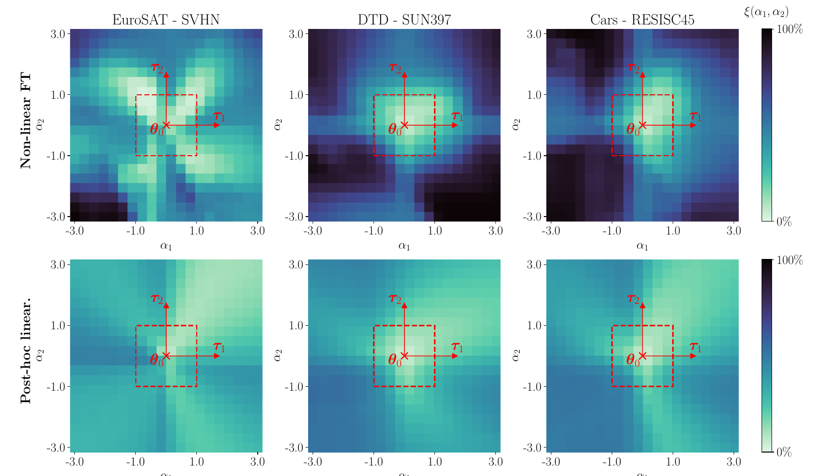
The center of each plot is the pretrained weights , and the two red arrows are the two task vectors. In the top row, the non-linear model is light only in a small patch near the origin, and the error climbs quickly once goes beyond 1. This explains two empirical observations in the original task arithmetic paper, that the best coefficient is usually below 1 and that fine-tuning calls for a small learning rate and few steps.
In the bottom row, the post-hoc linearized model has a much larger light region. Linearization makes task vectors interfere less with one another, which is why its normalized accuracy is higher.
Now the problem is clear. The linearized model disentangles well but is too weak on individual tasks; the non-linear model is strong on individual tasks but disentangles less well. Can we have both?
Fine-tuning directly in the tangent space
The authors' answer is to skip linearizing after the fact and instead fine-tune the linearized model from the very beginning.
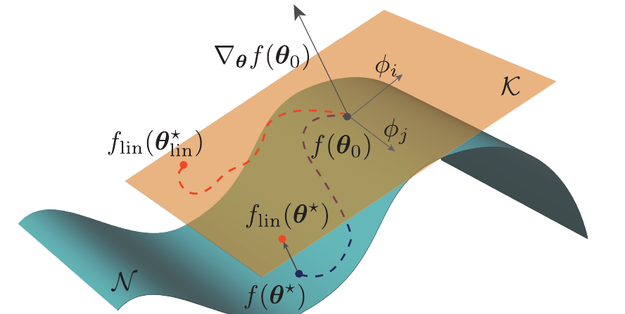
This figure puts the three approaches side by side. The curved surface is the set of all network functions, and the plane is the tangent space at . Standard fine-tuning travels along the surface to . Post-hoc linearization projects that endpoint onto the plane, which is why it loses accuracy. Linearized fine-tuning stays on the plane from start to finish, and what it optimizes for is the best point on the plane, .
The two linear models share the same kernel, but the task vector is optimized directly for the linear model, so its single-task performance is much better.
In practice, a linearized model is a network that “keeps fixed and trains the displacement.” PyTorch's torch.func.jvp computes both and the Jacobian times the displacement in a single forward pass. Let's use a small MLP to see when the linear approximation is accurate:
import torch
from torch.func import functional_call, jvp

torch.manual_seed(0)
net = torch.nn.Sequential(torch.nn.Linear(4, 16), torch.nn.Tanh(), torch.nn.Linear(16, 2))
theta0 = {k: v.detach().clone() for k, v in net.named_parameters()}
x = torch.randn(8, 4)

def f(params):
    return functional_call(net, params, (x,))

def f_lin(params):
    delta = {k: params[k] - theta0[k] for k in params}
    out, dp = jvp(f, (theta0,), (delta,))     # f(θ0) and J·(θ − θ0), both from a single forward pass
    return out + dp

direction = {k: torch.randn_like(v) for k, v in theta0.items()}
for scale in [0.01, 0.1, 1.0]:
    theta = {k: theta0[k] + scale * direction[k] for k in theta0}
    gap = (f(theta) - f_lin(theta)).abs().max().item()
    print(f"displacement scale {scale:<4}  max gap between original and linearized model {gap:.5f}")
displacement scale 0.01  max gap between original and linearized model 0.00152
displacement scale 0.1   max gap between original and linearized model 0.13638
displacement scale 1.0   max gap between original and linearized model 8.19715
With a small displacement the two are nearly identical; as the displacement grows, the gap widens fast. The linear model has no say in where standard fine-tuning ends up. Linearized fine-tuning instead ties the model to the tangent space, so however far it travels, the relationship between weights and outputs stays linear.
In the paper's experiments, the authors linearize only CLIP's image encoder; the text encoder is frozen anyway. The training setup is exactly that of standard fine-tuning, with 2,000 steps, batch size 128, learning rate and AdamW with a cosine schedule, and no extra hyperparameter tuning.
Discussion
Addition and subtraction both improve
The last row is linearized fine-tuning:
| Task addition (absolute/normalized %) | ViT-B/32 | ViT-B/16 | ViT-L/14 |
|---|---|---|---|
| Non-linear fine-tuning | 71.4/76.5 | 75.5/80.0 | 85.1/88.8 |
| Linearized fine-tuning | 76.5/85.4 | 81.3/86.0 | 88.5/93.5 |
Mean absolute accuracy after adding the eight tasks rises by 5.1, 5.8 and 3.4 percentage points for the three models.
Task forgetting is evaluated by subtracting a task vector and seeing how low the target task can be pushed while the control task, ImageNet, keeps at least 95% of its pretrained accuracy. On ViT-B/32, non-linear fine-tuning pushes the target task down to 24.0% and linearized fine-tuning to 10.9%, forgetting 13.1 percentage points more; on ViT-L/14 the figure goes from 18.0% to 7.9%. Accuracy on the control task is almost the same.
Coefficients are chosen as in the original paper, with a single shared by all tasks, searched from 0 to 1 in steps of 0.05, and the best value picked on a small portion of the training data.
The benefit of linearization is largest for small models and shrinks as models grow. The appendix also finds that larger models are more disentangled to begin with.
The cost
Linearization does not come free. The appendix explains that at inference, every operation needs an extra derivative computation, so it takes about two to three times as long as the original model; during training, the computation and memory for gradients roughly double. The authors describe this as “only a constant-factor increase,” but for large models, two to three times the inference cost shows up directly in deployment.
Later research picked up from exactly this point. Partial Linearization, for example, linearizes only LoRA's adapters, confining the cost to a small fraction of the parameters.
Why disentanglement happens
The authors close with an explanation from the kernel-method point of view. A kernel can be decomposed into a set of eigenfunctions . If each task uses only eigenfunctions that are “nonzero only inside its own input domain,” different tasks will not interfere with one another.
They check this on ViT-B/32. After linearized fine-tuning on RESISC45, they eigendecompose its NTK and compute the total energy of the eigenfunctions at each input point. RESISC45 data points have clearly higher energy, while Cars data points, used as a control, have very low energy. The eigenfunctions that represent RESISC45 really are concentrated on RESISC45's data.
The authors also explain that this localization is not a necessary condition for task arithmetic, because eigenfunctions might cancel each other out in other regions. It becomes necessary only when the eigenfunctions are linearly independent within each region.
Disentanglement is learned in pretraining
The last experiment takes pretraining away. Starting from a randomly initialized ViT, the authors fine-tune separately on each of the eight tasks to get task vectors, then add them together.
Task arithmetic fails completely. For ViT-B/32 from random initialization, non-linear fine-tuning gives a mean single-task accuracy of 48.5%, but after the eight vectors are added only 5.5% is left, about the same as a randomly initialized model with no fine-tuning (5.3%). Linearized fine-tuning behaves the same way.
So weight disentanglement emerges during pretraining. Pretraining does more than learn features that keep different meanings apart; it also keeps apart the weight directions that control those semantic regions.
The scope of the evidence
The main experiments all use CLIP ViTs and eight image classification datasets; the appendix adds T5 and convolutional networks. “Non-overlapping input domains” across tasks is the premise of the whole definition, and it roughly holds for these eight datasets. When two tasks' inputs overlap from the outset, as with two kinds of labels on the same text, this analysis cannot be applied directly.
Conclusion
The paper first refutes the claim that “task arithmetic comes from linear fine-tuning,” then formulates the condition task arithmetic needs as weight disentanglement, meaning that each task vector affects only its own input domain.
Linearized models disentangle better but are too weak on individual tasks. Move fine-tuning itself into the tangent space and you get the benefits of both, at the cost of two to three times the inference time.
If your deployment budget can absorb that multiple and you often need to add a pile of task vectors together, linearized fine-tuning is worth a try. The official code wraps the linearized model as a standard nn.Module, so training scripts need almost no changes.
If the budget can't take it, no problem. Just keep the coefficient at 1 or below. Past 1, the task vectors start fighting one another.