Original paper
2 OLMo 2 Furious
- Publication
- Publication venue not yet verified
- First submitted to arXiv
- arXiv:2501.00656
Cite this paper · BibTeX
The citation identifies the linked source version. It cites the original paper and its authors.
@misc{transformersolmo22024,
  title = {{2 OLMo 2 Furious}},
  author = {Team OLMo and Pete Walsh and Luca Soldaini and Dirk Groeneveld and Kyle Lo and Shane Arora and Akshita Bhagia and Yuling Gu and Shengyi Huang and Matt Jordan and Nathan Lambert and Dustin Schwenk and Oyvind Tafjord and Taira Anderson and David Atkinson and Faeze Brahman and Christopher Clark and Pradeep Dasigi and Nouha Dziri and Allyson Ettinger and Michal Guerquin and David Heineman and Hamish Ivison and Pang Wei Koh and Jiacheng Liu and Saumya Malik and William Merrill and Lester James V. Miranda and Jacob Morrison and Tyler Murray and Crystal Nam and Jake Poznanski and Valentina Pyatkin and Aman Rangapur and Michael Schmitz and Sam Skjonsberg and David Wadden and Christopher Wilhelm and Michael Wilson and Luke Zettlemoyer and Ali Farhadi and Noah A. Smith and Hannaneh Hajishirzi},
  year = {2024},
  eprint = {2501.00656},
  archivePrefix = {arXiv},
  url = {https://arxiv.org/abs/2501.00656}
}
The report's title is a joke, a play on the film title 2 Fast 2 Furious.
The content, though, is serious. OLMo is the family of "fully open" language models from the Allen Institute for AI (AI2). Each release includes not only the weights but also the pretraining data, training code, intermediate checkpoints, and training logs. Models like these matter for research: if you want to study training dynamics or the relationship between data and memorization, only fully open models will do. But their performance has always trailed open-weight models by some distance.
OLMo 2 aims to close that gap. It comes in three sizes, 7B, 13B, and 32B, trained on up to 6.6T tokens, and its post-training applies the same team's Tülu 3 recipe directly. The report focuses on four things: pretraining stability, the mid-training recipe, post-training, and infrastructure.
This note looks mainly at the first two. The first is what makes it possible for OLMo 2 to scale up at all; the second makes use of model merging.
Defining the problem
The previous version, OLMo-0424, performed within expectations, but its training was far from steady.
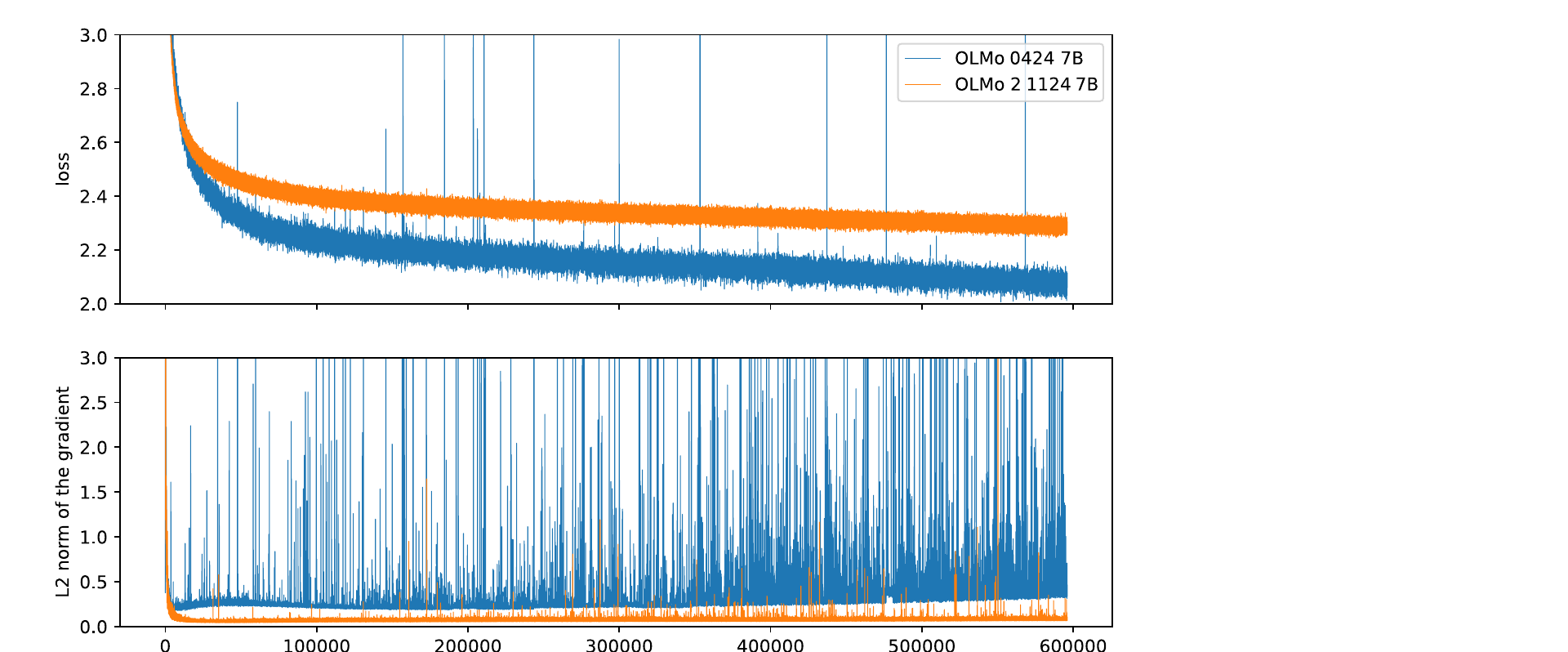
Blue is OLMo-0424, and it has two problems. The first is sudden spikes in the loss and the gradient norm, with gradient spikes often appearing before loss spikes. The second is that the baseline of the gradient norm slowly grows over the course of training, and the spikes become more and more frequent along with it. The authors found that the larger the model, the more spikes there are; together, the two eventually make training diverge, so scaling up is simply impossible.
Orange is OLMo 2, with the gradient staying almost flat along the bottom. The orange loss in the top plot looks higher because the two runs used different data, so they cannot be compared directly.
So which changes turned the blue line into the orange one?
Solving the problem
Seven changes for stability
The authors made seven changes in all. Some touch the data, some the architecture, and some just change a single hyperparameter.
1. Filtering repeated n-grams. Inspecting the batches where spikes occurred, the authors often found repeated fragments such as g400g400g400g400... or a long string of 255, 255, 255, .... The relationship is not certain: the same fragment triggers spikes in large models but not in small ones, and changing the data order may make the problem go away. Overall, though, removing this kind of data lowers the frequency of spikes.
In data curation, documents containing an n-gram repeated 32 or more times (n from 1 to 13 tokens) are deleted; the training code checks again when loading data and masks out the loss on anything that slipped through. This clearly reduces gradient spikes, but does nothing for the slow rise of the gradient norm.
2. Initialization. OLMo-0424 used scaled initialization, with smaller initial values in deeper layers. OLMo 2 goes back to the simplest approach and samples every parameter from a normal distribution with mean 0 and standard deviation 0.02. The authors measured how much activations and gradients grow or shrink from the first layer to the last in randomly initialized models; the new initialization keeps the scale more constant across different depths and widths.
3. RMSNorm. The parameter-free LayerNorm is replaced with RMSNorm.
4. Where normalization goes. This is a less common choice. Standard Pre-LN normalizes the input first and then sends it into the attention or feedforward layer; OLMo 2 instead normalizes the sublayer's output:
This approach comes from Swin Transformer V2. The residual stream itself is not normalized, but the increment each layer adds is first squeezed to a fixed scale, so no layer can suddenly add a very large value.
5. QK-norm. Before computing attention, RMSNorm is applied to the queries and keys, keeping attention logits from growing too large.
6. Z-loss. The loss gets an extra term , where is the denominator of the output-layer softmax. If the logits as a whole keep growing, grows with them, and this term pulls it back.
This term came with a side story. The FlashAttention library's cross-entropy implementation has z-loss built in, and the authors wrote a separate PyTorch version as a backup. The two gave identical forward passes but different backward passes, which the authors suspect comes down to numerical precision. Neither the training loss nor downstream performance showed any effect, yet the authors still threw away the stretch of training run with the swapped implementation, went back to where the two diverged, and reran it with the original. Midway through a run, they avoid swapping any implementation if they can.
7. Two optimizer settings. The embedding layer no longer gets weight decay, and AdamW's drops from to . The latter makes gradient norms lower and more stable early in training.
None of these seven changes is a new invention. The authors' contribution is to run the experiments one by one, measure each change's effect in OLMo's setting, and then put them all into a single recipe.
Two-stage pretraining
OLMo 2's pretraining has two stages.
Stage 1 takes more than 90% of training compute and uses OLMo 2 Mix 1124, about 3.9T tokens. Over 95% of it is web data (mainly from DCLM), and the rest is code (StarCoder), papers (peS2o, arXiv), math web pages, and Wikipedia. Code data keeps only repositories with at least 2 GitHub stars; documents in which the single most frequent word makes up more than 30% of the text are also deleted, to remove binary or almost entirely numeric content.
Stage 2, which the authors call mid-training, takes 5% to 10% of compute. The learning rate decays linearly to 0 in this stage, and the data switches to the curated Dolmino Mix 1124: the top 7% of web pages selected by a quality classifier, decontaminated FLAN instruction data, papers, Wikipedia, Stack Exchange Q&A, plus synthetic data specifically to shore up math ability.
The effect is large. After mid-training, the 7B model's average score on development evaluations rose by 10.6 points, surpassing a 13B that had finished only stage 1. GSM8K rose from 24.1 to 67.5, MMLU from 59.8 to 63.7, and DROP from 40.7 to 60.8.
Screening data with small anneals
How should mid-training data be chosen? A full 50B-token anneal is too expensive, so the authors devised a cheap method they call a microanneal.
- Pick one math data source, or a small group of them, to evaluate.
- Take an equal number of tokens from general data to form a small mix that is half math and half general data.
- Train on this small mix as an anneal, with the learning rate decaying linearly to 0 over its length.
They ran 19 microanneals, 130B tokens in total, which is fewer than three full 50B anneals, and differences usually showed up in under 10B tokens of training. The idea closely resembles the way Llama 3 uses annealing to evaluate small datasets, only done more systematically.
Model soups in mid-training
Next comes the step this note cares about most. Rather than run mid-training only once, the authors ran it several times on the same data with different data orders, then averaged the results.
To verify that this helps, the authors compared six mid-training mixes on 7B. Each mix was run with three different data orders for 50B tokens apiece, and they compared "the best of the three runs" with "all three averaged":
| Mix | Evaluation | Best single model | Average of three |
|---|---|---|---|
| A | OLMES | 75.6 | 77.0 |
| B | OLMES | 75.3 | 77.3 |
| C | OLMES | 76.3 | 76.8 |
| A | MMLU | 61.2 | 62.0 |
| B | MMLU | 61.5 | 62.7 |
| C | MMLU | 62.8 | 63.5 |
Across six mixes and four kinds of evaluation, 24 comparisons in all, the averaged model is no worse than the best single model in 23, and is usually better; for example, mix B gains 2 points on OLMES. The exception is mix E on GSM*, where averaging drops the score from 60.5 to 43.0.
So every final OLMo 2 model is a "soup." 7B averages three models each run for 50B tokens. 13B and 32B average four: three run for 100B tokens each and one run for 300B tokens, which the authors found works better than averaging only the three 100B runs.
It is worth setting this against Tülu 3. At the SFT stage, the same team averaged models with different seeds and found them no better than the best single model; in mid-training, averaging models with different data orders works in almost every case. The difference is that each mid-training model saw more than 50B tokens, and all of them started from the same pretraining checkpoint and decayed the learning rate to 0, conditions very close to the settings studied in Model Soups and PMA. The paper does not directly compare these two results; the explanation here is only a conjecture.
Post-training
Post-training largely copies Tülu 3: SFT, length-normalized DPO, and RLVR. There are two changes. Preference data now uses responses generated by permissively licensed models, and RLVR is run in multiple stages for the best performance.
Discussion
The Pareto frontier of compute and performance
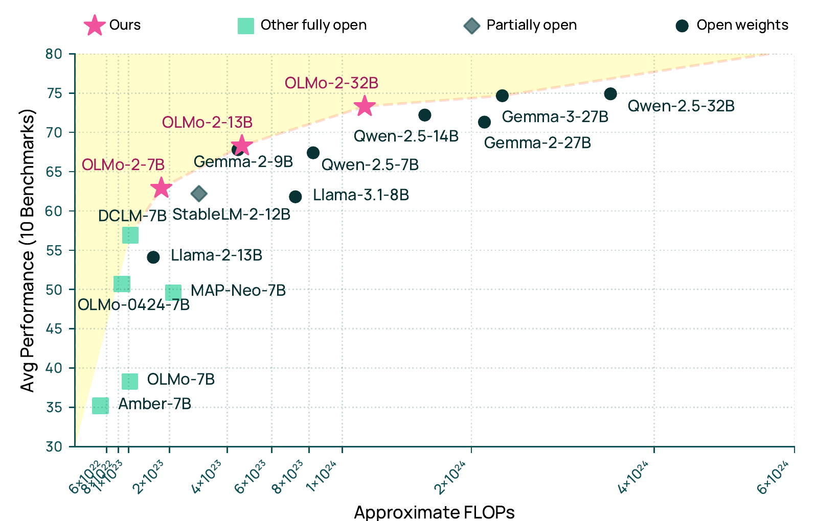
The horizontal axis is pretraining compute, and the vertical axis is the base models' average over 10 benchmarks. The pink stars sit on the dashed line toward the upper left: for the same compute, OLMo 2 performs better, or, for the same performance, it uses less compute. For example, OLMo 2 13B and Gemma 2 9B score about the same, while Qwen 2.5 7B used more compute to reach roughly the same spot.
The green squares are other fully open models, mostly in the lower left, and OLMo 2 has pulled well ahead of them.
For the post-trained versions, here are the average scores from the report's Table 7:
| Model | Average | Pretraining FLOPs () |
|---|---|---|
| OLMo 2 7B Instruct | 56.5 | 1.8 |
| Llama 3.1 8B Instruct | 59.1 | 7.2 |
| Qwen 2.5 7B Instruct | 61.6 | 8.2 |
| OLMo 2 13B Instruct | 63.5 | 4.6 |
| OLMo 2 32B Instruct | 68.8 | 13.0 |
| Qwen 2.5 32B Instruct | 68.1 | 35.0 |
| GPT-4o mini | 65.7 | — |
7B still trails Llama 3.1 8B and Qwen 2.5 7B, but with only about a quarter of their pretraining compute. 32B, with less than 40% of Qwen 2.5 32B's compute, gets a slightly higher average score and also surpasses GPT-4o mini.
Things to watch for when reading this report
- The evidence for stability is mostly a comparison of training curves in a single setting. The seven changes went in together, and only some of their individual contributions are ablated.
- How GSM8K was handled. When the authors found that math ability after pretraining was poor, they took 200 of GSM8K's 1,319 problems as a development set for mid-training, so GSM8K is not an entirely unseen evaluation. The report's final results use only the remaining 1,119 problems, and the authors state this explicitly in a footnote.
- The evidence for model soups comes from 7B mid-training at 50B tokens. For the four-model combinations of 13B and 32B, the report says only that they were "empirically better," with no complete table.
Conclusion
OLMo 2 is a very down-to-earth engineering report. It brings no new architecture; instead it gets stability, data mixing, and evaluation methods right one by one, and puts a fully open model on the compute-efficiency frontier for the first time.
For model merging, it offers a clean positive case: same starting point, same data, different data orders, averaged after annealing, and the result is almost never worse than the best single run.
If you have spare compute, don't bet everything on a single data order. Run mid-training a couple more times and average the results; you get more out of that than out of picking the best run.