Original paper
Exploring the Limits of Transfer Learning with a Unified Text-to-Text Transformer
- Publication
- Journal of Machine Learning Research 2020Journal
- First submitted to arXiv
- arXiv:1910.10683
Cite this paper · BibTeX
The citation identifies the linked source version. It cites the original paper and its authors.
@misc{transformerst52019,
  title = {{Exploring the Limits of Transfer Learning with a Unified Text-to-Text Transformer}},
  author = {Colin Raffel and Noam Shazeer and Adam Roberts and Katherine Lee and Sharan Narang and Michael Matena and Yanqi Zhou and Wei Li and Peter J. Liu},
  year = {2019},
  eprint = {1910.10683},
  archivePrefix = {arXiv},
  url = {https://arxiv.org/abs/1910.10683}
}
In the second half of 2019, there were more NLP pretraining papers than anyone could read.
BERT used masked language modeling, GPT-2 a left-to-right language model, XLNet permutation language modeling, and RoBERTa said BERT just hadn't been trained enough. Every paper changed several things at once: the objective, the architecture, the pretraining data, the number of training steps, the fine-tuning procedure. Scores went up in the end, but it was hard to say which change deserved the credit.
In this paper, Raffel, Shazeer and colleagues at Google did something brute-force and very expensive. They rewrote every task into the same format, fixed a baseline setup, and then changed one factor at a time, comparing them item by item. Once the comparisons were done, they combined the best choice for each item and scaled up to 11 billion parameters trained on about 1 trillion tokens (a behemoth in 2019, merely a small model today).
The authors say up front that the goal is not to propose a new method but to take stock of where the whole field stands. The unified model is called T5 (Text-to-Text Transfer Transformer). The paper also released a cleaned-up web corpus, C4, which later became pretraining data for many language models.
Defining the problem
In NLP, transfer learning means pretraining on large amounts of unlabeled text, then fine-tuning on labeled data for downstream tasks. By 2019, every stage of this pipeline had several options, and they were hard to compare with one another.
Encoder-only models like BERT are good at classification or at marking where the answer sits in the source text, but they can't directly generate a translation or a summary. Language models like GPT can generate, but for classification they usually need a separate classification head attached. Whenever the model, the loss function or the decoding method differs, any difference you measure is mixed up with other variables.
So the authors needed a common framework that handles classification, question answering, translation and summarization alike, so that the same model, the same loss function and the same set of hyperparameters could run every task. Only with that in place could they change one factor at a time.
Solving the problem
Text in, text out
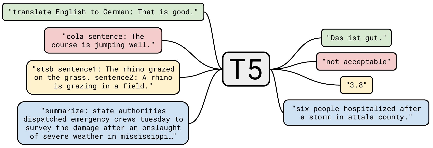
Every task is rewritten as “take in some text, output some text,” with the task name written in front of the input as a prefix. For translation, the input is “translate English to German: That is good.” and the model is trained to output “Das ist gut.”
Classification tasks work the same way, except that the output is the class name. MNLI asks for the relationship between a premise and a hypothesis, and the input is:
mnli premise: I hate pigeons. hypothesis: My feelings towards pigeons are filled with animosity.
The target output is the word entailment. If the model outputs a word that isn't one of the options, say “hamburger,” it simply counts as wrong; the authors say they never actually saw this happen.
Two kinds of tasks need a bit more conversion. STS-B asks for the similarity of two sentences as a real number from 1 to 5. The authors noticed that most labels come in increments of 0.2, so they round each score to the nearest 0.2 and turn it into a string; 2.57, for example, becomes “2.6”, and the regression problem becomes a 21-class classification. For Winograd-style pronoun disambiguation tasks, the ambiguous pronoun is marked with asterisks, and the model is asked to output the noun it refers to:
Input: The city councilmen refused the demonstrators a permit because *they* feared violence.
Output: The city councilmen
Every task is trained with maximum likelihood, that is, ordinary cross-entropy with teacher forcing. The wording of the prefix is itself a kind of hyperparameter; the authors tried rephrasing it and found it made little difference.
The model: close to the original Transformer
The model is a standard encoder-decoder Transformer, with only three changes:
- LayerNorm only rescales, with no additive bias.
- LayerNorm moves to the input of each sublayer, and the residual path itself isn't normalized; this is what later came to be called Pre-LN.
- Relative position encoding is simplified to a scalar added directly to the attention logits. Each attention head has its own set, shared across all layers. There are 32 buckets in total, whose distance ranges grow logarithmically, and every distance beyond 128 goes into the same bucket. A single layer can't tell positions apart beyond 128, but a stack of layers can.
The output layer shares weights with the input embedding, the same as in the original Transformer. The authors didn't ablate these three changes, since they're unrelated to the factors the paper sets out to compare.
The baseline model's encoder and decoder each have 12 layers, and each is about the size of BERT-Base, with , a feed-forward size of , and 12 attention heads with each. That's about 220 million parameters in total, roughly twice BERT-Base, since there are two stacks.
C4: cleaned-up web text
Common Crawl scrapes about 20TB of web text every month, but most of it is menus, error messages, repeated boilerplate or code. The authors applied a series of rules to the April 2019 snapshot:
- Keep only lines that end in a period, exclamation mark, question mark or closing quotation mark.
- Discard any page with fewer than 3 sentences; keep only lines with at least 5 words.
- If a page contains any word from a “bad words list,” delete the whole page.
- Delete lines containing “Javascript” and pages containing “lorem ipsum.”
- Delete pages containing a curly brace
{, since that's usually code. - Remove Wikipedia citation markers, as well as lines containing strings like “terms of use” or “cookie policy.”
- Deduplicate: for any three-sentence span that appears more than once, keep only one copy.
- Use langdetect to keep only pages with at least a 0.99 probability of being English.
The result is about 750GB, which the authors named the Colossal Clean Crawled Corpus, or C4 for short. More than three years later, when Meta trained LLaMA, C4 still made up 15% of the pretraining data.
Baseline training setup
Pretraining runs for steps with batches of 128 sequences of length 512; after packing, each batch holds about tokens, for a total of about billion tokens. That's far fewer than BERT's roughly 137 billion or RoBERTa's roughly 2.2 trillion, but enough to compare settings, and C4 is big enough that no data is repeated over the whole run.
The optimizer is AdaFactor. Pretraining holds the learning rate at 0.01 for the first steps, then decays it with the inverse square root of the step count. Every downstream task is fine-tuned for steps at a constant learning rate of 0.001, with a checkpoint saved every 5,000 steps, and the best checkpoint on the validation set is reported. The vocabulary is 32,000 wordpieces trained with SentencePiece on a 10:1:1:1 mix of English C4 and German, French and Romanian, since there are translation tasks for those three languages downstream.
The pretraining objective: predict only the dropped-out spans
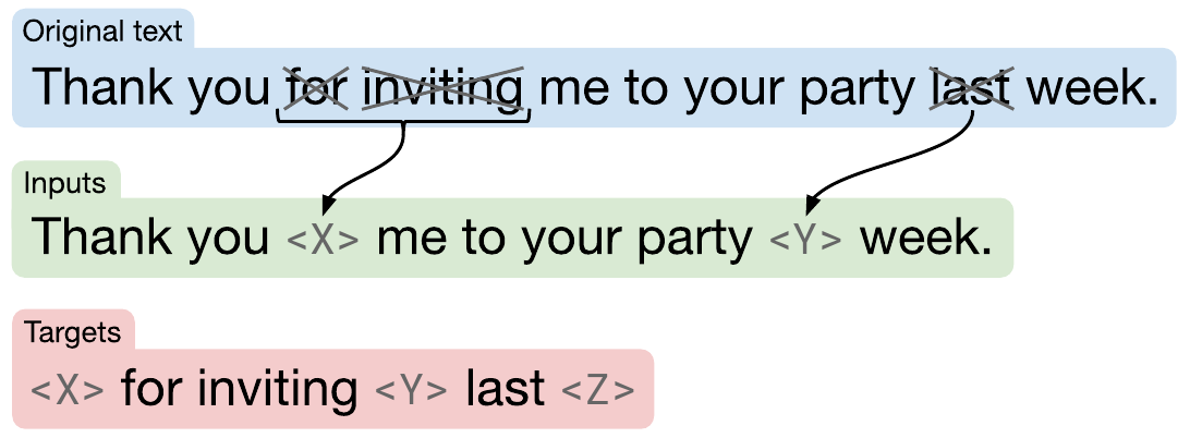
The baseline objective is adapted from BERT's masked language modeling. Randomly pick 15% of the tokens to corrupt; consecutive selected tokens merge into one span, which is replaced by a single “sentinel” token, with a different sentinel for each span. The output contains only the dropped-out spans, each preceded by the same sentinel that replaced it, plus one final sentinel to mark the end.
Let's write out the example from the figure:
tokens = "Thank you for inviting me to your party last week .".split()
noise = [0, 0, 1, 1, 0, 0, 0, 0, 1, 0, 0]  # 1 = token selected for corruption

def span_corrupt(tokens, noise):
    sentinels = iter(["<X>", "<Y>", "<Z>"])
    inputs, targets, prev = [], [], 0
    for tok, n in zip(tokens, noise):
        if n and not prev:          # start of a corrupted span: insert a sentinel
            s = next(sentinels)
            inputs.append(s)
            targets.append(s)
        if n:
            targets.append(tok)     # corrupted tokens appear only in the output
        else:
            inputs.append(tok)
        prev = n
    targets.append(next(sentinels))  # one final sentinel to mark the end
    return inputs, targets

inputs, targets = span_corrupt(tokens, noise)
print(" ".join(inputs))    # Thank you <X> me to your party <Y> week .
print(" ".join(targets))   # <X> for inviting <Y> last <Z>
print(len(tokens), len(inputs), len(targets))  # 11 10 6
“for” and “inviting” are adjacent, so they share one <X>. The original sentence has 11 tokens; the input is down to 10 and the output has only 6. If you followed BERT and had the model “output the whole original sentence” instead, the decoder would have to generate 11 tokens. The authors chose to predict only the dropped-out spans mainly to save computation; the shorter the decoder's sequence, the faster pretraining goes.
The actual T5 uses special tokens such as <extra_id_0> and <extra_id_1> as sentinels; they're added to the vocabulary and don't correspond to any wordpiece.
How stable is the baseline?
Repeating every experiment many times would be too expensive. Instead, the authors trained the baseline setup from scratch 10 times and used the standard deviation of those 10 runs as the reference for every variant. For most tasks the standard deviation is under 1% of the score; small datasets like CoLA, CB and COPA are the exceptions. CB's validation set has only 56 examples, and its F1 standard deviation reaches 3.2. The paper's tables put in bold every result within two standard deviations of the best score.
Train the same model for steps without pretraining, and GLUE drops from 83.28 to 66.22 and SQuAD from 80.88 to 50.31. English–French translation is barely affected (39.82 vs. 39.77), because that dataset is large enough on its own.
Discussion
The body of the paper is a long series of controlled experiments, covering architecture, objectives, data, training strategy and scaling. The tables report the average GLUE and SuperGLUE scores, ROUGE-2 for CNN/DM summarization, exact match for SQuAD, and BLEU for the three translation pairs, all on validation sets except for the final results.
Architecture: count parameters and compute separately
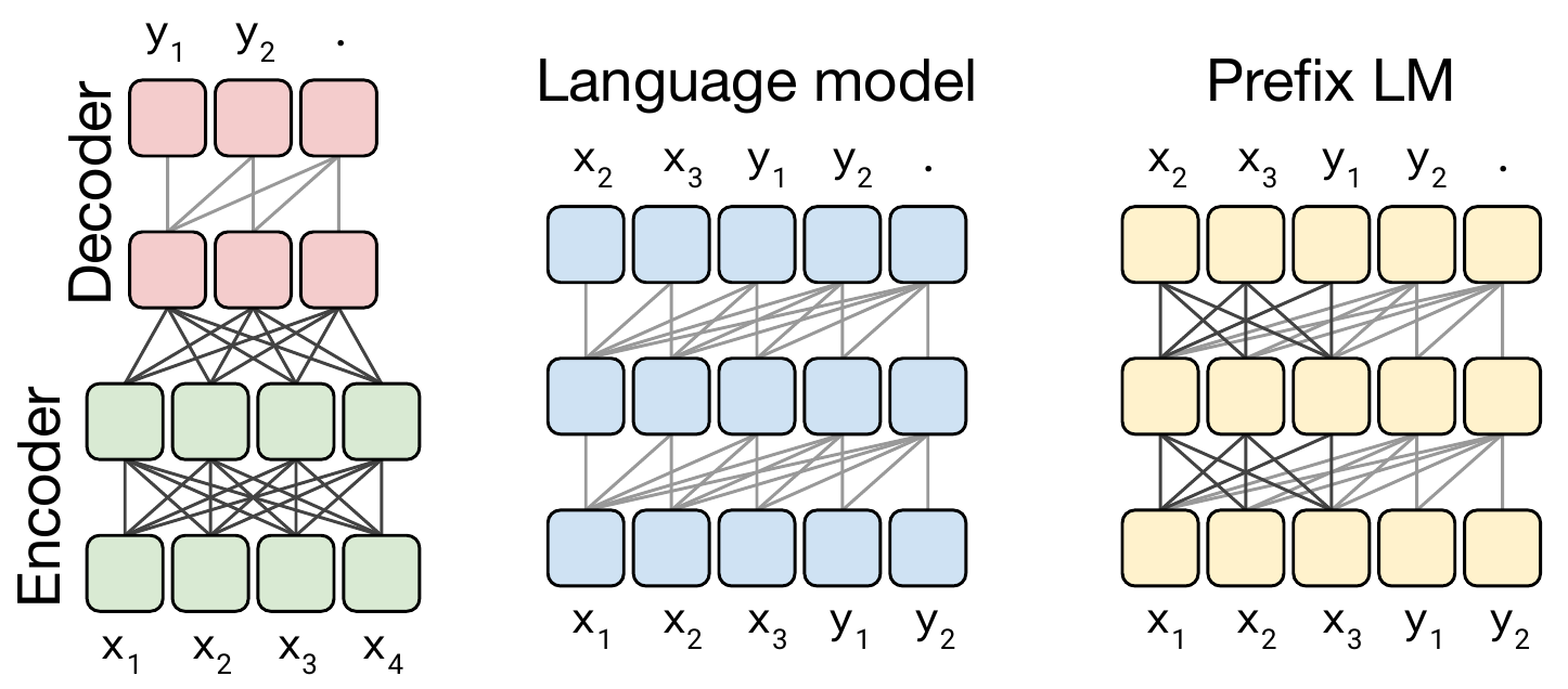
In the figure, dark gray lines mean fully visible attention and light gray lines mean a causal mask, where each position can only look at earlier positions. To handle translation, a language model has to join the input and output into one sequence: “translate English to German: That is good. target: Das ist gut.” The problem is that the causal mask also restricts every position in the input to looking only at what came before it, so the representation of the earlier part of the sentence can't see the later part. The prefix LM fixes this by making the input portion fully visible. On classification tasks, a prefix LM is actually a lot like BERT; the only difference is that the classification result is generated directly by the output layer.
Before comparing architectures, you have to decide what counts as “fair.” A model whose encoder and decoder each have layers has about as many parameters as a -layer language model, but its compute is only comparable to an -layer language model, because the encoder processes only the input and the decoder only the output, whereas a language model runs every layer over the input plus the output. In the authors' measurements, the two take almost exactly the same time per step.
Let a BERT-Base-sized stack have parameters and need FLOPs to process one input–output pair. Here are the results:
| Architecture | Objective | Params | Compute | GLUE | SuperGLUE | SQuAD | En–De BLEU |
|---|---|---|---|---|---|---|---|
| Encoder-decoder | Denoising | 83.28 | 71.36 | 80.88 | 26.98 | ||
| Encoder-decoder, shared parameters | Denoising | 82.81 | 70.73 | 80.63 | 26.72 | ||
| Encoder-decoder, 6 layers each | Denoising | 80.88 | 68.42 | 77.59 | 26.38 | ||
| Language model | Denoising | 74.70 | 55.02 | 61.14 | 25.09 | ||
| Prefix LM | Denoising | 81.82 | 68.11 | 78.94 | 26.43 | ||
| Encoder-decoder | Language modeling | 79.56 | 64.29 | 76.02 | 26.27 |
Compiled from Table 2 of the paper, showing selected rows and columns.
For the same compute, the encoder-decoder with a denoising objective is best on every task. Sharing parameters between the encoder and decoder halves the parameter count and costs only a little in score, and it still beats a prefix LM with the same parameters; the authors credit the explicit encoder-decoder attention for this. Halving the number of layers, by contrast, clearly hurts. Another consistent result is that the denoising objective beats the language modeling objective on every architecture.
Pretraining objectives: small differences, so pick the cheap one
Objectives are compared in three rounds. The first round compares three broad approaches: prefix language modeling (GLUE 80.69), BERT-style masking (82.96), and shuffling a sentence then restoring it (73.17). BERT-style is best, and deshuffling lags well behind.
The second round compares BERT-style variants: dropping the random token replacement, replacing whole spans with sentinels, or simply deleting the corrupted tokens. All four variants score very close to one another. Deleting tokens outright comes out slightly higher on GLUE, mostly thanks to CoLA (60.04 against the baseline's 53.84); the authors guess that judging whether a sentence is grammatical has something to do with noticing where words are missing. On SuperGLUE, though, it does worse than the sentinel version.
The third round tunes the corruption rate and span length. Rates from 10% to 25% make little difference; at 50%, GLUE and SQuAD drop noticeably. Span corruption is described by two parameters. In a 500-token sequence, corrupting 15% means 75 tokens; if those must form 25 spans, each span averages 3 tokens. The version with mean span length 3 slightly beats corrupting individual tokens at random on most non-translation tasks (SuperGLUE 72.53 vs. 71.36), and its sequences are shorter, so it trains faster.
The authors conclude that among the denoising objectives they tried, the differences in performance are small, and the choice should be driven mainly by computational cost.
Pretraining data: filtering helps, too little leads to memorization
Remove all of C4's filtering rules (keeping only language detection), and the data grows to 6.1TB while every task gets worse; GLUE drops from 83.28 to 81.46.
Smaller, domain-focused data wins on specific tasks. Wikipedia plus the Toronto Books Corpus (the combination BERT used, 20GB in total) raises SuperGLUE to 73.24, almost entirely through MultiRC, whose exact match jumps from 25.78 to 50.93; MultiRC's largest data source happens to be fiction. The RealNews-like version, which keeps only content from news sites, raises the news reading comprehension task ReCoRD from 68.16 to 73.72. The closer the downstream task's domain is to the pretraining data, the better the results.
The price is data volume. Imitating GPT-2's WebText recipe (keeping only links with a Reddit score of at least 3) across 12 months of Common Crawl yields only 17GB. The authors also deliberately truncated C4 so that the same 34 billion tokens of training would loop over the same data repeatedly. At 64 repeats the effect is small; at 1,024 repeats, GLUE drops to 79.55; at 4,096 it drops to 76.34, while the training loss gets noticeably lower, a sign that the model has started memorizing the data.
Training strategy: fine-tuning all parameters is still best
Methods that update only some of the parameters come out behind. Adapters add a small “dense–ReLU–dense” block after each feed-forward layer and train only that block and the LayerNorms. With an inner dimension of , SQuAD still gets 79.32, but English–German translation falls to just 13.84 BLEU. Small adapters are enough for low-resource tasks, while high-resource tasks need a much larger dimension. Gradual unfreezing causes a small drop on every task.
In the text-to-text framework, multi-task learning just means mixing examples from different datasets into the same batch. The hard part is deciding how much of the mix each task should get. The authors compared three mixing strategies:
- Examples-proportional: the more data a task has, the more often it's sampled, but with a cap so that huge datasets like the unlabeled data and English–French translation don't drown out the other tasks.
- Temperature-scaled: raise each task's proportion to the power and renormalize; is the same as proportional mixing, and the larger is, the closer the mix gets to even.
- Equal: every task has the same probability of being sampled.
Equal mixing is worst, with GLUE at only 76.13. With proportional mixing, most tasks have a best ; for temperature scaling, works best. None of the mixing strategies, however, catches up with “unsupervised pretraining, then fine-tuning on each task separately.”
A compromise works. Pretraining on a multi-task mixture and then fine-tuning on each task gives GLUE 83.11, about the same as the baseline's 83.28, and slightly better English–Romanian translation. Leaving the target task out of the pretraining mixture (leave-one-out) lowers scores only slightly, which shows that a model that has seen many tasks can still adapt to one it hasn't seen. Pretraining only on labeled tasks, with no unlabeled data at all, is clearly worse on everything except translation.
Given 4× the compute, how should you use it?
With 4 times the compute, should you train longer, make the model bigger, or build an ensemble? The authors actually ran the comparison.
| Approach | GLUE | SuperGLUE | SQuAD | CNN/DM | En–De BLEU |
|---|---|---|---|---|---|
| Baseline | 83.28 | 71.36 | 80.88 | 19.24 | 26.98 |
| Same size, 4× training steps | 85.33 | 74.72 | 82.45 | 19.33 | 27.08 |
| Same size, 4× batch size | 84.60 | 74.64 | 82.52 | 19.42 | 27.07 |
| 2× model size, 2× training steps | 86.18 | 77.18 | 84.18 | 19.66 | 27.52 |
| 4× model size, same number of steps | 85.91 | 78.04 | 83.86 | 19.73 | 27.47 |
| Ensemble of 4 independently trained models | 84.77 | 71.74 | 83.09 | 20.10 | 28.05 |
Compiled from Table 13 of the paper, showing selected rows and columns.
All four approaches help. Making the model bigger is usually more effective than just adding training; a 2× model trained 2× as long and a 4× model come out about the same. The ensemble beats every other approach on CNN/DM summarization and on English–German and English–Romanian translation, but does almost nothing for SuperGLUE. The authors also point out that a bigger model makes later fine-tuning and inference more expensive, whereas the cost of training a small model longer can be amortized across many downstream tasks.
Putting it together: T5
The final T5 combines the study's conclusions:
- Objective: span corruption, with 15% of tokens corrupted and a mean span length of 3.
- Training volume: 1 million steps with batches of sequences of length 512, about 1 trillion tokens, 32 times the baseline. The domain-focused datasets are too small and would be repeated hundreds of times, so C4 is still used.
- Model sizes: Small (60 million), Base (220 million), Large (770 million), 3B and 11B. 3B and 11B mainly scale up the feed-forward layers, with of 16,384 and 65,536 and with 32 and 128 attention heads, respectively. The authors say they widened the feed-forward layers because TPUs are best at large dense matrix multiplications.
- Multi-task pretraining followed by fine-tuning, with GLUE and SuperGLUE now fine-tuned one subtask at a time and the batch size cut to 8 to keep the small datasets from overfitting.
- Translation and summarization switch to beam search with a beam width of 4.
T5 set the state of the art at the time on 18 of the 24 tasks. The 3B model already beat previous work on a few tasks, and the authors consider scaling to 11B the most important step in getting the best results. GLUE averages 90.3; SuperGLUE averages 88.9, against a previous best of 84.6 and a human score of 89.8; SQuAD exact match is 91.26, against a previous best of 90.1. ROUGE-2 on CNN/DM is 21.55, against a previous best of 20.30.
Behind the scores are problems the authors point out themselves. T5 beats humans by a wide margin on MultiRC and ReCoRD, which the authors think more likely reflects metrics that favor machine outputs; humans score 100% on both COPA and WSC, and T5 still falls well short there. It didn't win a single translation task. Pretraining used only English, while the best translation systems of the time also used data augmentation such as back-translation.
The last experiment answers how much of T5's improvement is just scale. The baseline model trained on the same 1 trillion tokens (Baseline-1T) scores GLUE 84.80, SuperGLUE 73.90 and SQuAD 83.01; T5-Base scores 85.97, 75.64 and 85.44. The two have the same size and the same amount of training, differing only in the non-scaling changes selected during the study, and T5-Base wins on every task.
Later scrutiny
C4 was widely used after its release, and in 2021 Dodge et al. produced the first fairly thorough documentation study of C4. The single domain contributing the most tokens is patents.google.com. The content includes machine-translated text as well as test items from other NLP benchmarks; for XSum summarization, for example, 15.49% of the reference summaries appear verbatim in C4.
They took a close look at what the bad-words list removed. Among the deleted documents, clusters dominated by sexual content make up about 30%; the rest include science, medicine and health documents as well as legal and political ones. After classification with a dialect topic model, documents in African American English and Hispanic-aligned English turned out to be removed at rates of 42% and 32%, against only 6.2% for White-aligned English. Documents mentioning sexual orientation were the most likely to be filtered out; in a manual check of removed documents related to “gay,” 36% were neither offensive nor sexual. Whole-page keyword filtering is cheap, but what it removes is not neutral.
The architecture conclusion is also worth checking against later work. T5's comparison was done in the “pretrain, then fine-tune on each task” setting. In 2022, Wang et al. at BigScience redid the comparison in a different setting. Looking only at zero-shot performance after pretraining, a causal decoder with an autoregressive language modeling objective is best; after adding multi-task prompted fine-tuning, an architecture with full visibility over the input trained with a masked objective is best. In other words, T5's conclusion holds in its own setting; the later shift of large models toward decoder-only architectures has to do with the growing emphasis on zero-shot and few-shot use.
Conclusion
This paper reads like a very long lab manual. First write every task as text in, text out, then change one factor at a time. From architecture, objectives and data to fine-tuning and scale, every factor has a table you can look up.
If you only want to take away a few points, they're roughly these. Denoising objectives are all about the same, so pick the one that's cheapest to train; clean the pretraining data first, and make sure there's enough of it that you never need to repeat it; and spend any extra compute on a bigger model first.
As for “encoder-decoder is best,” two years later not even Google's own PaLM followed it.