[17.06] Transformer

The Dawn of a New Era

Attention Is All You Need

---

Unlike previous sequential models, the Transformer model introduced a new era of self-attention mechanisms.

This model no longer relies on recursive calculations of sequences but instead uses attention mechanisms for sequence modeling, making the training and inference processes more efficient.

Defining the Problem

In past sequence modeling tasks, RNN and LSTM models were mainstream.

However, these models faced several issues during training and inference:

1. Limitations of Recursive Calculations

RNN and LSTM models need to calculate each element of the sequence step-by-step during training, leading to serialized computations that hinder efficient parallel processing.

2. Long-Distance Dependency Problem

Due to the recursive nature of RNN and LSTM models, they struggle to capture dependencies between distant positions in a sequence when processing long sequences.

Solving the Problem

Model Design

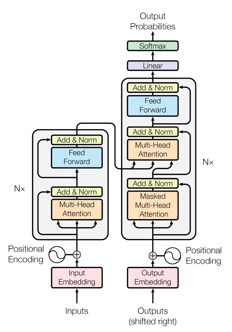
This is the Transformer model architecture diagram provided in the original paper.

Although this diagram is very concise (???), most people usually do not understand it at first glance.

Believe it or not, this is already simplified!

Let's write a simple code snippet to see how this model actually works:

Input Layer

Here, the input is a sequence of data, represented as a tensor.

• First dimension: Batch size, referred to as B.
• Second dimension: Sequence length, referred to as T.
• Third dimension: Feature dimension, referred to as D.

Let's start with a simple example:

input_text = ['你', '好', '啊', '。']
input_text_mapping = {
    '你': 0,
    '好': 1,
    '啊': 2,
    '。': 3
}

In this example, the input text is "你好啊。", with a total of 4 characters.

info

Here, we greatly simplify the entire training process to make it easier for you to understand.

Next, convert this input into a tensor:

import torch
import torch.nn as nn

input_tensor = torch.tensor([
    input_text_mapping[token]
    for token in input_text]
)
print(input_tensor)
# >>> tensor([0, 1, 2, 3])

Next, we embed each element:

embedding = nn.Embedding(num_embeddings=4, embedding_dim=512)
embedded_input = embedding(input_tensor)
print(embedded_input)
# >>> tensor([[ 0.1,  0.2,  0.3,  ...,  0.4],
#             [ 0.5,  0.6,  0.7,  ...,  0.8],
#             [ 0.9,  1.0,  1.1,  ...,  1.2],
#             [ 1.3,  1.4,  1.5,  ...,  1.6]])
print(embedded_input.shape)
# >>> torch.Size([4, 512])

tip

Embedding is not a complex technique; it simply projects each element into a higher-dimensional space using a linear transformation layer.

Finally, don't forget we need a 3D tensor as input, so we need to add a batch size dimension. In this example, the batch size is 1.

embedded_input = embedded_input.unsqueeze(0)
print(embedded_input.shape)
# >>> torch.Size([1, 4, 512])

Positional Encoding

In traditional RNN and LSTM models, the model captures sequence dependencies through the position of elements in the sequence.

Therefore, we do not need special positional encoding, as the model implicitly includes positional information in each iteration of the For-Loop.

However, the Transformer architecture lacks such implicit positional information; it only consists of linear transformation layers. In linear transformation layers, each element is independent with no intrinsic relationships. Hence, we need additional positional encoding to help the model capture positional dependencies in the sequence.

In this paper, the authors propose a simple positional encoding method using sine and cosine functions:

Let's implement a positional encoding function based on the above formula:

import math
import torch

def sinusoidal_positional_encoding(length, dim):
    """ Sinusoidal positional encoding for non-recurrent neural networks.
        REFERENCES: Attention Is All You Need
        URL: https://arxiv.org/abs/1706.03762
    """
    if dim % 2 != 0:
        raise ValueError(
            'Cannot use sin/cos positional encoding with '
            f'odd dim (got dim={dim})')

    # position embedding
    pe = torch.zeros(length, dim)
    position = torch.arange(0, length).unsqueeze(1)
    div_term = torch.exp(
        (torch.arange(0, dim, 2, dtype=torch.float) * -(math.log(10000.0) / dim)))
    pe[:, 0::2] = torch.sin(position.float() * div_term)
    pe[:, 1::2] = torch.cos(position.float() * div_term)

    return pe

This function considers both sequence length and feature dimensions, providing each position with a fixed positional encoding.

Let's visualize the positional encoding, assuming a sequence length of 256 and a feature dimension of 512:

import cv2
import numpy as np

pos_mask = sinusoidal_positional_encoding(256, 512)
pos_mask = pos_mask.numpy()
pos_mask = (pos_mask-pos_mask.max()) / (pos_mask.max()-pos_mask.min())
pos_mask = np.array(pos_mask * 255).astype(np.uint8)
pos_mask = cv2.applyColorMap(pos_mask, cv2.COLORMAP_JET)

tip

What is the significance of the number 10000 in the formula?

The number 10000 represents the scale of the positional encoding. By restricting the scale within a suitable range, it effectively captures the relationships between different positions while avoiding the adverse effects of excessively high or low frequencies.

If the number 10000 is changed to 100, the frequencies of the sine and cosine functions increase, causing positional encodings to repeat over shorter distances. This might reduce the model's ability to perceive relationships between distant positions as their encodings will appear more similar.

After obtaining the positional encoding, we need to add it to the input embedding tensor:

pos_emb = sinusoidal_positional_encoding(4, 512)
embedded_input = embedded_input + pos_emb

Self-Attention Mechanism

After obtaining the input encoding, we can move on to the core part of the Transformer model: the self-attention mechanism.

Here, we need to prepare three transformation matrices:

1. Query Matrix W_q.

   First, declare a set of weights W_q, then multiply the input embedding tensor by the Query matrix to get the Query tensor.

   W_q = nn.Linear(512, 512)
   query = W_q(embedded_input)
   print(query.shape)
   # >>> torch.Size([1, 4, 512])

2. Key Matrix W_k.

   Similarly, declare a set of weights W_k, then multiply the input embedding tensor by the Key matrix to get the Key tensor.

   W_k = nn.Linear(512, 512)
   key = W_k(embedded_input)
   print(key.shape)
   # >>> torch.Size([1, 4, 512])

3. Value Matrix W_v.

   Finally, declare a set of weights W_v, then multiply the input embedding tensor by the Value matrix to get the Value tensor.

   W_v = nn.Linear(512, 512)
   value = W_v(embedded_input)
   print(value.shape)
   # >>> torch.Size([1, 4, 512])

So, what exactly is this QKV stuff?

You can think of the transformation matrices as projections.

Projections mean "viewing from a different perspective."

The QKV process involves three different projections of the input, followed by the self-attention mechanism calculations.

---

The second step of the self-attention mechanism is to calculate the attention scores.

In this step, we perform a dot product between the Query tensor and the Key tensor.

attn_maps = torch.matmul(query, key.transpose(-2, -1))
print(attn_maps.shape)
# >>> torch.Size([1, 4, 4])

This gives us an attention score matrix of size 4x4.

In this example, it explores the relationships between [你, 好, 啊, 。] (you, good, ah, .).

In the formula, you'll see 1/sqrt(d_k), which scales the attention scores to prevent them from becoming too large or too small.

attn_maps = attn_maps / math.sqrt(512)

Next is the Softmax operation:

attn_maps = F.softmax(attn_maps, dim=-1)

tip

Why use Softmax? Why not Sigmoid?

The Softmax function converts all attention scores into a probability distribution, ensuring the total attention score sums to 1. This allows better weighting of

each position. Additionally, the Softmax function has a competition mechanism, enabling the model to differentiate between positions more effectively.

After calculating the attention map, we can perform a weighted sum of the Value tensor:

attn_output = torch.matmul(attn_maps, value)
print(attn_output.shape)
# >>> torch.Size([1, 4, 512])

Finally, apply residual connections:

attn_output = embedded_input + attn_output

Multi-Head Attention Mechanism

After understanding the above section, your next question might be: "What if we want multiple attention scores instead of just one for each position?"

The authors also thought of this, so they proposed the multi-head attention mechanism.

In the multi-head attention mechanism, we prepare multiple sets of QKV matrices and perform self-attention calculations for each set.

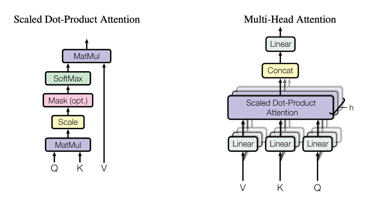
Although the concept is to have multiple heads, in practice, we do not prepare multiple sets of QKV matrices. Instead, we split the original QKV matrices into multiple sub-matrices and perform self-attention calculations on each sub-matrix, like this:

# Split into multiple heads
Q = Q.view(Q.size(0), Q.size(1), self.num_heads, self.head_dim).transpose(1, 2)
K = K.view(K.size(0), K.size(1), self.num_heads, self.head_dim).transpose(1, 2)
V = V.view(V.size(0), V.size(1), self.num_heads, self.head_dim).transpose(1, 2)

However, this is too engineering-focused and does not introduce new concepts, so we will not delve deeper here.

Cross-Attention Mechanism

In the Transformer architecture, the attention mechanisms in the Encoder and Decoder are similar but have some differences.

In the Encoder, we perform self-attention calculations for each position in the sequence; in the Decoder, besides self-attention calculations for each position, we also need to perform attention calculations on the Encoder's output, which is known as cross-attention.

The Decoder consists of two parts: the first part performs self-attention on its own sequence, and the second part performs cross-attention on the Encoder's output. We have covered self-attention; now let's discuss cross-attention calculations.

Again, we need to prepare three transformation matrices:

1. Query Matrix W_q.

   First, declare a set of weights W_q, multiply the Decoder's input embedding tensor by the Query matrix to get the Query tensor. The length of decoder_input can be different from encoder_output. If we encounter a translation problem, this length might be 10.

   W_q = nn.Linear(512, 512)
   decoder_query = W_q(decoder_input)
   print(decoder_query.shape)
   # >>> torch.Size([1, 10, 512])
   tip

   Here, the input is decoder_input.

2. Key Matrix W_k.

   Similarly, declare a set of weights W_k, multiply the Encoder's output embedding tensor by the Key matrix to get the Key tensor.

   W_k = nn.Linear(512, 512)
   encoder_key = W_k(encoder_output)
   print(encoder_key.shape)
   # >>> torch.Size([1, 4, 512])
   tip

   Here, the input is encoder_input.

3. Value Matrix W_v.

   Finally, declare a set of weights W_v, multiply the Encoder's output embedding tensor by the Value matrix to get the Value tensor.

   W_v = nn.Linear(512, 512)
   encoder_value = W_v(encoder_output)
   print(encoder_value.shape)
   # >>> torch.Size([1, 4, 512])
   tip

   Here, the input is encoder_input.

The subsequent steps are the same as the self-attention mechanism: first, calculate the attention map:

attn_maps = torch.matmul(decoder_query, encoder_key.transpose(-2, -1))
print(attn_maps.shape)
# >>> torch.Size([1, 10, 4])

Then, perform scaling and Softmax:

attn_maps = attn_maps / math.sqrt(512)
attn_maps = F.softmax(attn_maps, dim=-1)

Finally, perform a weighted sum of the Value tensor:

attn_output = torch.matmul(attn_maps, encoder_value)
print(attn_maps.shape)
# >>> torch.Size([1, 10, 4])
print(encoder_value.shape)
# >>> torch.Size([1, 4, 512])
print(attn_output.shape)
# >>> torch.Size([1, 10, 512])

info

In the self-attention phase of the Decoder, a mask operation is typically added to ensure that during decoding, future information cannot be seen. This mask is usually an upper triangular matrix, ensuring that the Decoder can only see the generated part during decoding.

def _generate_square_subsequent_mask(
    sz: int,
    device: torch.device = torch.device(torch._C._get_default_device()),  # torch.device('cpu'),
    dtype: torch.dtype = torch.get_default_dtype(),
) -> Tensor:
    r"""Generate a square causal mask for the sequence.

    The masked positions are filled with float('-inf'). Unmasked positions are filled with float(0.0).
    """
    return torch.triu(
        torch.full((sz, sz), float('-inf'), dtype=dtype, device=device),
        diagonal=1,
    )

Feed-Forward Network

After the self-attention mechanism, we need to pass through a simple feed-forward network to extract features.

ffn = nn.Sequential(
    nn.Linear(512, 2048),
    nn.ReLU(),
    nn.Linear(2048, 512)
)
ffn_output = ffn(attn_output)
output = attn_output + ffn_output
print(output.shape)
# >>> torch.Size([1, 4, 512])

This feed-forward network is a typical fully connected network. Here, we use two fully connected layers with a ReLU activation function in between.

Additionally, there is an expand-dim operation in the module, usually with an expansion factor of 4. This operation is similar to the concept of the Inverted Residual Bottleneck Block proposed in MobileNet-V2. The main purpose is to improve the model's nonlinear representation ability by expanding the dimensions and then compressing them.

Layer Normalization

We haven't mentioned LayerNorm yet.

This operation is straightforward. After understanding all the steps above, it just takes a few lines of code.

In each step, we should apply LayerNorm to each output. There are two types: Norm-First and Norm-Last, depending on your model architecture. We will discuss this in more detail in other papers.

norm1 = nn.LayerNorm(512)
attn_output = norm1(embedded_input + attn_output)

# ...

norm2 = nn.LayerNorm(512)
output = norm2(attn_output + ffn_output)

tip

Why not use Batch Normalization?

Sequence data relies more on its characteristics than those of batch data. Therefore, LayerNorm is more suitable than BatchNorm in this context.

Discussion

Why Use Self-Attention?

In short, it's fast.

---

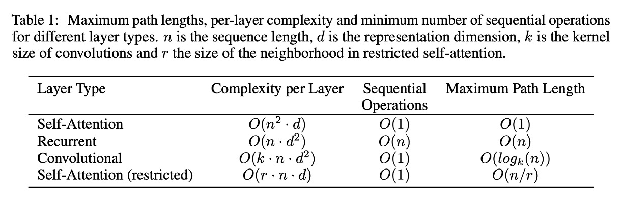
The authors summarized the computational complexity of RNN, CNN, and Self-Attention, as shown in the figure above.

1. Self-Attention Layer (Unrestricted):

   • Per Layer Complexity: O(n^2·d): In the self-attention mechanism, each input token (sequence length n) needs to attend to every other token, forming an (n * n) attention matrix. Each matrix element requires calculations based on the embedding dimension (d), resulting in a total complexity of O(n^2·d).
   • Sequential Operations: O(1): The full attention matrix can be computed in parallel, allowing all comparisons to occur simultaneously.
   • Maximum Path Length: O(1): Since each token can directly attend to any other token, the maximum path length is just one step.

2. RNN:

   • Per Layer Complexity: O(n·d^2): RNN layers process each token sequentially. Each token's calculation combines the current token embedding (d-dimension) and the hidden state (also d-dimension), resulting in an operation cost of O(d^2). Since n tokens are processed, the total complexity is O(n·d^2).
   • Sequential Operations: O(n): Due to RNN's sequential nature, each token must wait for the previous token's calculation to complete before processing the next.
   • Maximum Path Length: O(n): In RNNs, the path length between two tokens requires traversing through all intermediate tokens between them.

3. CNN:

   • Per Layer Complexity: O(k·n·d^2): In convolutional layers, a kernel of width k slides over the sequence to compute local features. Each n tokens need computations in the d-dimensional embeddings, and each convolution operation costs O(d^2). Thus, the total complexity is O(k·n·d^2).
   • Sequential Operations: O(1): Each convolution filter can be applied to the entire sequence simultaneously.
   • Maximum Path Length: O(log_k(n)): By stacking convolutional layers with dilation, the network can connect distant tokens logarithmically to k.

4. Restricted Self-Attention Layer:

   • Per Layer Complexity: O(r·n·d): Here, each token can only attend to a neighborhood of size r. The attention matrix becomes (n·r), but each element still requires calculations based on the embedding dimension (d), resulting in a total complexity of O(r·n·d).
   • Sequential Operations: O(1): Similar to unrestricted self-attention, all comparisons can be performed simultaneously.
   • Maximum Path Length: O(n/r): Since each token can only attend to a smaller neighborhood, the path length between two distant tokens increases to O(n/r).

Experimental Results: Machine Translation

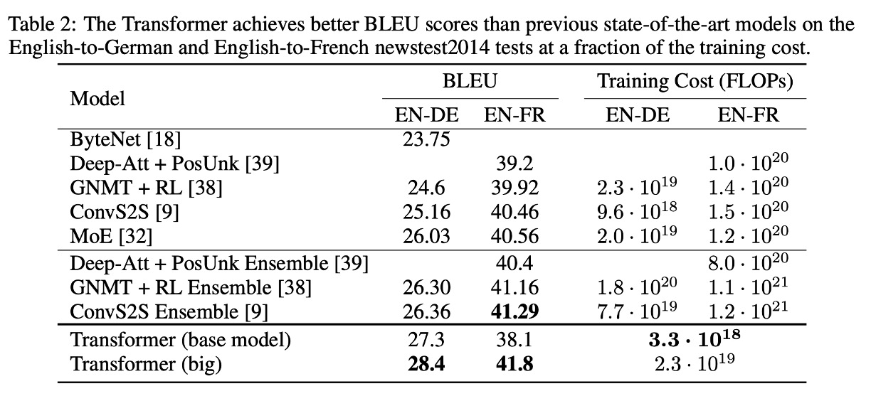
In the WMT 2014 English-German translation task, the Transformer (big) improved the BLEU score by over 2.0 points compared to the previous best models (including ensemble models), setting a new record of 28.4 BLEU. This model trained for 3.5 days using 8 P100 GPUs. Even the base model surpassed all previously published models and ensemble models at a significantly lower training cost.

In the WMT 2014 English-French translation task, the Transformer (big) achieved a BLEU score of 41.0, outperforming all previously published single models at a quarter of the training cost.

Conclusion

The Transformer is a groundbreaking architecture that not only addresses some of the issues of RNN and LSTM models but also improves training and inference efficiency.

When first introduced, the Transformer architecture did not make a significant impact.

While the Transformer was widely and continuously discussed in academic circles for several years, from natural language processing to computer vision, it might have only attracted the attention of engineers and researchers in the industry.