Original paper
Unifying Short and Long-Term Tracking with Graph Hierarchies
- Publication
- CVPR 2023Conference
- First submitted to arXiv
- arXiv:2212.03038
Cite this paper · BibTeX
The citation identifies the linked source version. It cites the original paper and its authors.
@misc{multiobjecttrackingsushi2022,
  title = {{Unifying Short and Long-Term Tracking with Graph Hierarchies}},
  author = {Orcun Cetintas and Guillem Brasó and Laura Leal-Taixé},
  year = {2022},
  eprint = {2212.03038},
  archivePrefix = {arXiv},
  url = {https://arxiv.org/abs/2212.03038}
}
Tracking through a long video really means solving a whole series of problems at different time scales.
Between two adjacent frames, people barely move, and position alone is enough to match them. Someone blocked for half a second who then reappears needs a motion model to push the estimate forward. Someone blocked for over ten seconds before walking back out no longer lines up with any position, and only appearance can identify them again.
The best trackers of the time mostly chained several methods together, using a Kalman filter or Tracktor for the short term and hanging a ReID module on for the long term. Graph neural network methods were in the same situation. MPNTrack handles only 15 frames at a time, and its public detections first have to go through Tracktor.
Guillem Brasó and Laura Leal-Taixé of the Technical University of Munich are the very authors of MPNTrack. This time, together with Orcun Cetintas, they wanted to know whether a single model could handle everything from two adjacent frames all the way to frames five hundred apart.
Defining the problem
The authors compare the common trackers of the time with four diagrams.

The authors see two problems with hybrid approaches like (c).
The first is scale. When association is done with a graph, each edge is the hypothesis "these two detections belong to the same person." To let detections frames apart be linked too, edges have to connect every pair of frames, and the number of edges grows with the square of the number of detections.
The labels are even more of a problem. Each detection has at most two correct edges, one to the past and one to the future. With detections, there are at most correct edges, while the total number of edges can reach . As the detections pile up, the share of correct edges approaches zero, and the network sees almost nothing but negatives.
The second is generality. Which cue to use at each time scale is decided in advance by engineers. But different datasets need different cues. In DanceTrack, everyone dresses identically and the frame rate is high, so position and motion are more reliable than appearance; BDD is shot from driving cars with a lot of camera shake, so there only appearance holds up. Every new kind of scene means retuning the combination.
Solving the problem
Stacking up level by level
SUSHI recursively splits a long clip into small time windows, and each level connects edges only within a window.
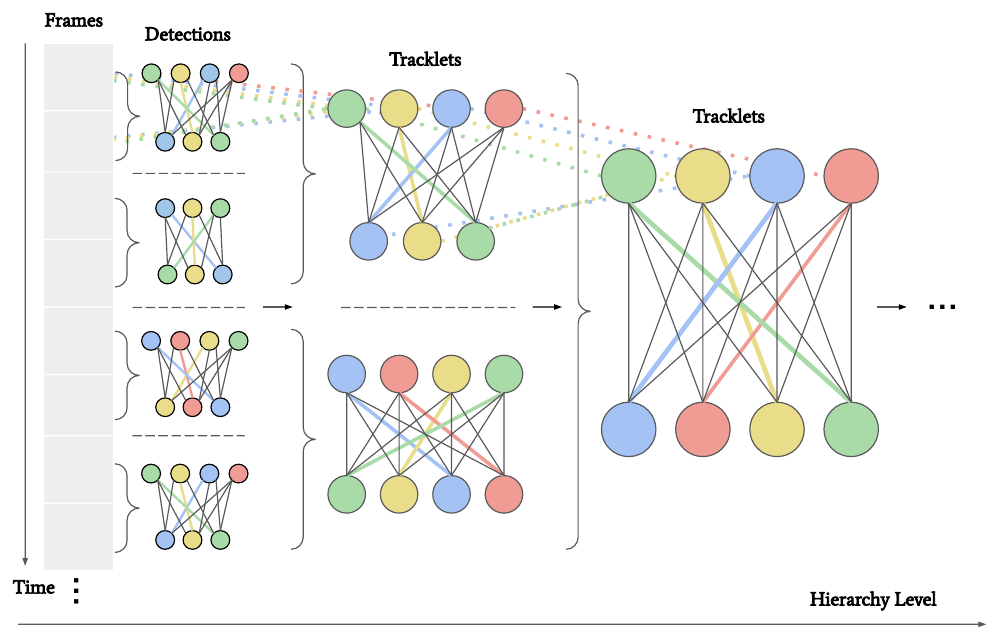
At the first level, each window has only two frames, and the detections in the two adjacent frames are linked, giving tracklets of length 2. At the second level the windows have four frames, the nodes become the previous level's tracklets, and these are merged into longer ones. The window at level covers frames, so after nine levels a window is 512 frames. On MOT17, that's roughly 17 to 36 seconds.
Each level up, there are fewer nodes, but the edges can span longer stretches of time.
Counting edges with an example
Let's use an idealized example to see how many edges the hierarchy saves.
Take a 512-frame clip with 20 people in every frame, everyone detected, and every level merging correctly. No pruning yet.
- One big graph. Between every two frames there are edges. There are 130,816 ways to pick two of the 512 frames, for a total of 52,326,400 edges.
- A nine-level hierarchy. Each window is made of two sub-windows, each with 20 tracklets, so there are only 400 candidate edges between them. The number of windows across the nine levels is , for a total of 204,400 edges.
Both approaches have the same number of correct edges to pick out in the end, , since each person has 512 detections and chaining them into one path takes 511 edges.
| Approach | Edges | Correct share |
|---|---|---|
| One big graph | 52,326,400 | 0.02% |
| Nine-level hierarchy | 204,400 | 5% |
Worked example for this note.
There are 256 times fewer edges, and the share of correct edges goes from two in ten thousand up to five percent. The former decides whether it fits on a GPU; the latter decides whether the network can learn at all.
The actual model prunes edges once more, connecting each node only to its 10 nearest neighbors. A single big graph needs a very large number of neighbors to avoid pruning away correct edges; in the small graphs, 10 is enough.
Every level is the same block
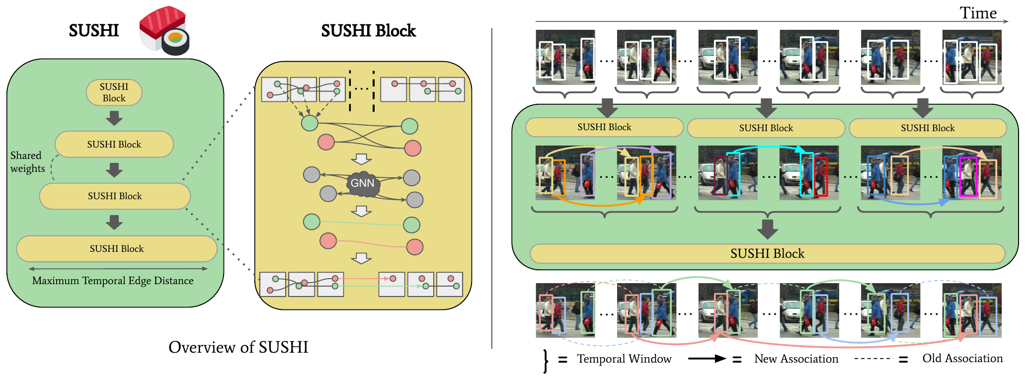
Each level is called a SUSHI block, and what it does inside is the same as MPNTrack:
- Take the previous level's tracklets as nodes, and connect edges between tracklets at different times within the window.
- Use MPNTrack's time-aware message passing to let nodes and edges exchange information for several rounds. Nodes aggregate the edges from the past and from the future separately.
- Use a small MLP to decide whether each edge links the same person.
- Round the scores with linear programming, ensuring each node has at most one edge forward and one backward, then merge the linked tracklets.
Edges start with four kinds of features. Position, size and time distance are computed from the two detections, one per tracklet, that are closest in time. Appearance uses the average ReID feature of all the detections in a tracklet, which is more stable than a single detection's.
The fourth is motion, which MPNTrack doesn't have. A single detection has no velocity, but a tracklet does. Project the earlier tracklet's last position forward in time and the later tracklet's first position backward, to the time point midway between them, then compute the GIoU of the two projected boxes. Projecting from both ends toward the middle, each side only has to predict across half the time.
Nine levels, one set of weights
The paper's most crucial design choice is that the nine SUSHI blocks share not only the same architecture but the same weights.
The data the different levels see varies a lot. At the first level, two nodes are only one frame apart; at the ninth, they may be hundreds of frames apart. To let the model know which level it's at, the authors learn a level embedding for each level and add it to the edges' initial embeddings.
Sharing weights lets data from all nine levels train the same network, multiplying the samples several times over; convergence is faster and there are fewer parameters. Excluding the ReID network, the whole model has only about 22K parameters.
More importantly, which cue to look at for which time scale is no longer decided by people. When the same network sees edges with large position gaps and long time gaps, it learns by itself to switch to appearance.
During training, each upper level's input is the output of the level below. While the lower levels haven't learned well yet, the tracklets the upper levels receive are wrong. So the authors start from the first level and unfreeze one more level every 500 iterations, then train all nine together once they're all unfrozen. Each level computes its own focal loss, and the losses are summed.
At inference, a 512-frame sliding window is used with 256 frames of overlap each time; tracks that share the most detections in the overlap are treated as the same track and stitched together with bipartite matching. Given the detections, it runs at 21 fps on MOT17.
Discussion
One network at every level
The ablations use three-fold cross-validation on the MOT17 training set. The authors compare four time spans, focusing on IDF1:
| Span | Hybrid | IDF1 | SUSHI | IDF1 |
|---|---|---|---|---|
| 25 frames | Tracktor | 65.6 | — | — |
| 75 frames | MPNTrack++ | 73.2 | 2 levels | 73.5 |
| 150 frames | MPNTrack++ | 73.4 | 3 levels | 74.8 |
| 512 frames | MPNTrack++ | 73.7 | 9 levels | 77.6 |
Compiled from Table 1 of the paper, three-fold cross-validation on the MOT17 training set.
MPNTrack++ is MPNTrack plus SUSHI's motion features, with the short term still left to Tracktor. Stretching the hybrid approach from 75 frames to 512 adds only 0.5 IDF1; SUSHI climbs all the way from 73.5 to 77.6.
The long-term stage of the hybrid approach is always a single graph. Stretch the time and the graph grows, and the label imbalance described earlier gets worse with it.
Clip length and number of levels
| Clip length | 1 level | 3 levels | 5 levels | 7 levels | 9 levels |
|---|---|---|---|---|---|
| 8 frames | 64.1 | 65.9 | — | — | — |
| 32 frames | 64.2 | 70.0 | 71.3 | — | — |
| 128 frames | 61.9 | 75.1 | 75.6 | 75.8 | — |
| 512 frames | — | 76.2 | 76.8 | 77.1 | 77.6 |
Compiled from Figure 4(b) of the paper, MOT17 training set, IDF1.
With only one level, clips longer than 32 frames actually do worse, dropping to 61.9 at 128 frames. The graph is too big and there are too many negatives for the network to learn. Add levels, and the longer the clip, the better. Nine levels on 512 frames reaches 77.6, 13.4 above the best single-level result of 64.2.
What each level looks at
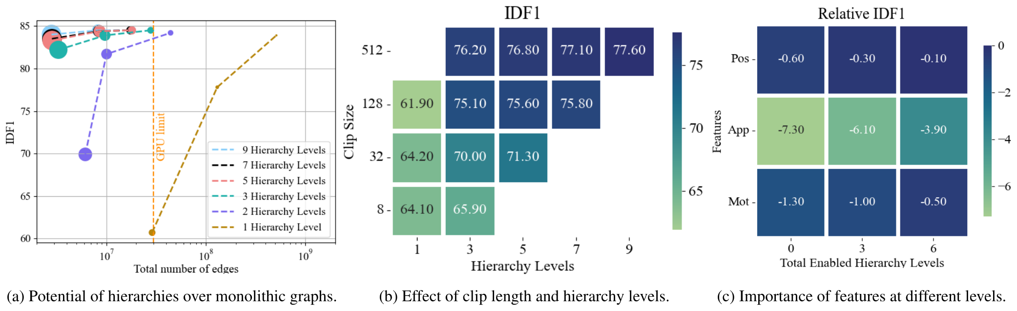
(c) checks whether the same network relies on different cues at different levels.
- Appearance matters most, and mainly at the higher levels. Switching it off everywhere costs 7.3 IDF1. Switching it off only at levels 7 to 9 costs 3.9; keeping it only at levels 1 to 3 recovers just 1.2 over switching it off everywhere.
- Motion has about the same effect at every level. Switching it off everywhere costs 1.3, a moderate effect.
- Position only helps at the low levels. Switching it off everywhere costs only 0.6, and keeping it in the first three levels recovers half of that.
For adjacent frames, look at position; once they're far apart, look at what people look like, which matches intuition. The difference is that the network learned this from data by itself, without anyone writing the rules for it.
Four datasets
| Dataset | Rival | IDF1 | HOTA | SUSHI IDF1 | HOTA |
|---|---|---|---|---|---|
| MOT17 public | MPNTrack | 61.7 | 49.0 | 71.5 | 54.6 |
| MOT17 private | ByteTrack | 77.3 | 63.1 | 83.1 | 66.5 |
| MOT20 private | ByteTrack | 75.2 | 61.3 | 79.8 | 64.3 |
| DanceTrack | ByteTrack | 53.9 | 47.7 | 63.4 | 63.3 |
Compiled from Tables 2–4 of the paper, test sets.
In the MOT17 public-detection setting, SUSHI uses exactly MPNTrack's network, yet its IDF1 is 9.8 higher; the only difference is the hierarchy. With ByteTrack's YOLOX detections, IDF1 is 5.8 higher, and ID switches fall from 2,196 to 1,149, nearly halved.
DanceTrack improves the most, with HOTA jumping from ByteTrack's 47.7 to 63.3, also above MOTR and QDTrack (both 54.2), the highest HOTA among the other methods in the paper's table. ByteTrack is strong on both MOT17 and MOT20 but falls behind on DanceTrack; SUSHI leads on all three datasets. On BDD, shot from driving cars, SUSHI simply applies the same GNN to eight classes, and mIDF1 on the test set rises from 55.8 to 60.0.
MOTA is a different story. On MOT20, SUSHI's MOTA is 74.3, lower than ByteTrack's 77.8. What SUSHI improves is association; missed detections and false positives are beyond its reach.
Limitations
SUSHI is an offline method. It needs a whole 512-frame clip before it can start, so it can't be used in systems that need real-time output. The 21 fps is also the speed once detections have already been computed.
The ReID network is off the shelf and not fine-tuned on tracking data, so all of SUSHI's improvement comes from the association side. In the public-detection setting, like other graph methods, it first refines the detection boxes with Tracktor, and that step is itself a short-term tracker.
Conclusion
SUSHI doesn't invent a new graph network; every level is MPNTrack. It swaps one huge, sparse graph for nine small graphs stacked on top of one another. The edges drop by two orders of magnitude, the share of correct edges climbs back from two in ten thousand to five percent, and the network can finally learn.
Shared weights, meanwhile, hand "which cue for which time scale" back to the data. The same network looks at position at the low levels and at appearance at the high levels, with nobody telling it to.
Nine levels and 512 frames come to about half a minute on MOT17. For occlusions longer than that, it all comes down to whether the stitching between sliding windows holds.