Original paper
Learning a Neural Solver for Multiple Object Tracking
- Publication
- CVPR 2020Conference
- First submitted to arXiv
- arXiv:1912.07515
Cite this paper · BibTeX
The citation identifies the linked source version. It cites the original paper and its authors.
@misc{multiobjecttrackingmpntrack2019,
  title = {{Learning a Neural Solver for Multiple Object Tracking}},
  author = {Guillem Brasó and Laura Leal-Taixé},
  year = {2019},
  eprint = {1912.07515},
  archivePrefix = {arXiv},
  url = {https://arxiv.org/abs/1912.07515}
}
There's a lovely old idea in offline tracking, which is to draw all the detections in a video as one graph.
Each detection is a node, and an edge connects any two detections in different frames. If two detections belong to the same track and are next to each other in time, the edge is "active." Tracking then becomes a graph partitioning problem: find which edges should be active.
The standard approach in this framework has two steps. First, give each edge a cost that expresses how likely the two detections are to be the same person; then hand the costs to an optimization solver to find the best partition overall.
By 2019, research in this direction had roughly split into two camps. One put its effort into the form of the graph, designing ever more complex optimizations that brought in higher-order relationships, but the costs were mostly still hand-designed. The other used deep models such as Siamese networks to learn better edge costs and then passed them to a simple solver, but those costs looked only at pairs and couldn't see the whole scene.
Guillem Brasó and Laura Leal-Taixé at the Technical University of Munich felt that each road went only halfway. Leal-Taixé is one of the authors of MOT16 and Tracktor. This time, the two wanted to see whether a network could learn the "solving" step as well.
Defining the problem
Tracking written as network flow
The authors start from classic min-cost flow, with a few simplifications.
Given all the detections in a video, , each detection consists of the image inside the box, the box coordinates and a timestamp. Build an undirected graph with one node per detection, and connect any two detections in different frames with an edge. Allowing edges that skip frames means tracks with missed detections in the middle can be joined back up.
Each edge has a binary variable . If the two nodes belong to the same track and are adjacent detections on that track, ; otherwise it's 0.
Tracks can't share nodes, so has to satisfy two conditions. Each node connects to at most one active edge toward the past:
and at most one toward the future:
This is a simplified version of the network flow conservation constraints.
The traditional approach gives each edge a cost and solves
Under the two sets of constraints above, this problem can be solved optimally in polynomial time.
Predicting the answer directly
Since what's needed in the end is , the authors skip learning costs altogether and learn directly.
Each edge becomes a binary classification problem, with as the label. The whole tracking problem then turns into a task that can be trained end to end, with both the features and the "solution" learned in the same network.
The remaining problem is that a classifier looking at only two nodes can't learn global information such as "this person has already been linked to someone else." To let each edge's decision consider the whole graph, the authors use a message passing network (MPN).
Solving the problem
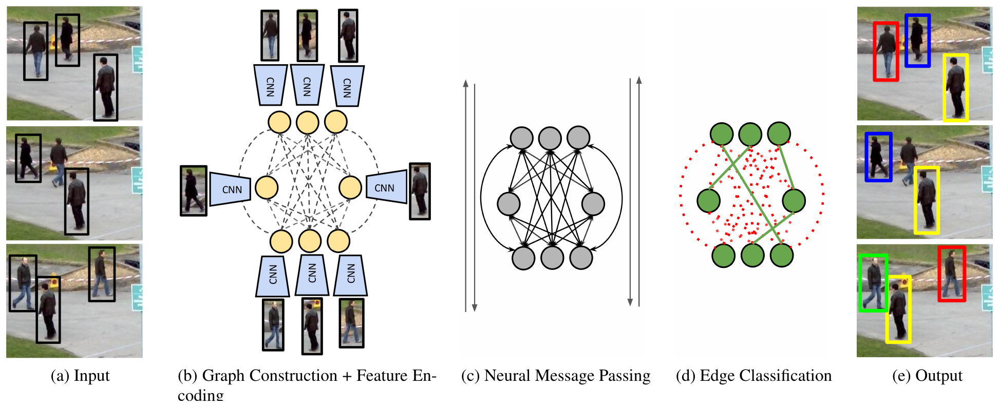
The whole process has four steps: building the graph, encoding features, message passing and edge classification.
Initial features
The initial node embeddings come from appearance. The authors take a ResNet-50 pretrained on ImageNet and train it on three person re-identification datasets, Market-1501, CUHK03 and DukeMTMC, to get 256-dimensional re-ID features; three fully connected layers then compress the node embedding to 32 dimensions.
The initial edge embeddings come from geometry. For two detection boxes in different frames, and , first compute their relative position and relative size:
Dividing the displacement by the average height of the two boxes lets people near and far be compared on the same scale. Add the time difference and the Euclidean distance between the two re-ID features, feed everything into an MLP, and you get the initial edge embedding.
Message passing
In an ordinary message passing network, each step has two updates. First, the edges are updated from the nodes at their two ends:
Then the nodes are updated from the edges connected to them. Each edge produces a message, and all the messages are summed (or averaged, or max-pooled) to get the new node embedding.
After repeating this times, every node and edge carries information from within a distance of , which works much like a CNN's receptive field. Edge classification, which used to look at just two boxes, can now see "what other candidates are around these two nodes."
Time-aware node updates
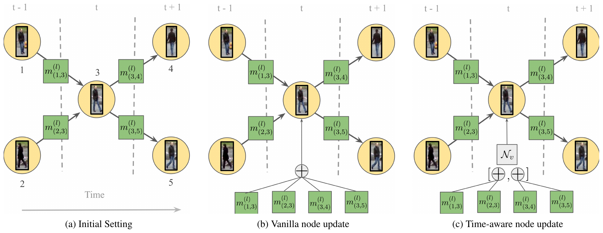
The paper's main architectural change is the node update.
Go back to the network flow constraints: each node connects to at most one edge toward the past and at most one toward the future. But an ordinary node update mixes the messages from all neighbors into one sum, and once they're summed, the node has no way of telling which messages came from the past and which from the future, so it's hard to judge whether the constraints are being violated.
The authors write the temporal structure of the MOT graph straight into the update rule. For node , messages from past and future neighbors are computed with two different MLPs. Past neighbors use
Future neighbors use instead. The two sides are summed separately into and , concatenated and fed into one last MLP:
The in the formula is the initial embedding, fed into every step so that the network doesn't forget the original features even after passing messages many times. The edge update is likewise fed the initial edge features.
Training and inference
The edge classifier is an MLP that outputs a single sigmoid value. From step to the final step , the edge embeddings at every step are used for prediction, and a weighted binary cross-entropy is computed over all of them:
where the loss for each edge at step is
Active edges are far rarer than inactive ones, so positive samples are multiplied by an extra weight .
At inference time, the final step's predictions are taken directly as the answer for and binarized at a threshold of 0.5. The network isn't forced to satisfy the network flow constraints, so after thresholding, a node may end up with two edges going out of it. The authors prepared two ways of fixing this: one greedily keeps only the highest-scoring edge, and the other uses linear programming to find the exact optimal rounding. In practice, very few edges violate the constraints, and the two methods barely differ; the greedy one's IDF1 is just 0.2 lower.
Implementation details
Here are a few settings that matter a lot once you actually run it:
- Frozen CNN. The authors found that training the ResNet along with everything else brought no clear improvement but cost much more compute, so all the convolutional layers are frozen and only the MLPs after them are trained.
- Sliding window. The video is cut into graphs of 15 frames each, with 14 frames of overlap between neighboring graphs; for overlapping edges, the predictions from the different graphs are averaged. Static-camera sequences are sampled at 6 frames per second and moving-camera ones at 9, so each graph covers only about one and a half to a little over two seconds of video.
- Pruning. Fully connecting nodes in different frames would make the number of edges explode, so two nodes are connected only if each is among the other's top 50 nearest neighbors by re-ID features.
- Preprocessing with Tracktor. The public detections are first run through Tracktor; the IDs it assigns are thrown away, and only its corrected boxes are kept as input. Tracktor's boxes are more accurate, and it also fills in some missed detections in neighboring frames. Frames missing in the middle of the output tracks are first filled from Tracktor's tracks, and whatever is still missing is filled by interpolation.
That last point deserves attention. MPNTrack's own network runs at 35 frames per second, but the Tracktor in front of it runs at only 8, so the whole system averages 6.5 frames per second.
Discussion
The ablations are all run on the MOT17 training set with three-fold cross-validation.
Time-aware updates
| Node update | MOTA ↑ | IDF1 ↑ | ID switches ↓ | Constraints met ↑ |
|---|---|---|---|---|
| Standard | 63.0 | 67.3 | 1,022 | 82.1% |
| Time-aware | 64.0 | 70.0 | 602 | 98.8% |
Compiled from Table 1 of the paper. Constraints met is the average share of network flow conservation constraints satisfied at a threshold of 0.5.
Separating past and future adds nearly 3 points of IDF1 and cuts ID switches from 1,022 to 602.
The last column is more interesting still. When the ordinary MPN's output is binarized directly, only 82.1% of the constraints are satisfied; the time-aware version reaches 98.8%. The network has almost learned the rule "each person links to only one forward and one backward" by itself, without needing an external solver to enforce it.
How many steps to pass
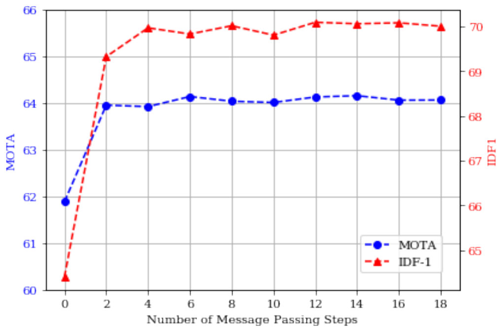
Zero steps means no message passing at all, just binary classification on the initial edge embeddings, which amounts to the traditional approach of "learning pairwise costs."
From 0 to 2 steps, MOTA and IDF1 both jump sharply; that's the step from pairwise to higher-order relationships. After that, the upward trend levels off around 6 steps, and there's no further improvement beyond 12. The final setting is .
Where the features come from
| Edge features | MOTA ↑ | IDF1 ↑ | FP ↓ | ID switches ↓ |
|---|---|---|---|---|
| Time difference only | 58.8 | 52.6 | 13,127 | 2,962 |
| Time + position | 63.6 | 68.7 | 6,308 | 895 |
| Time + position + appearance | 64.0 | 70.0 | 6,169 | 602 |
Compiled from Table 2 of the paper.
This table is a bit of a surprise. Adding relative position lifts IDF1 from 52.6 to 68.7, the biggest step; adding appearance features on top adds only 1.3 IDF1. But appearance pushes ID switches down further, from 895 to 602, so it's still worth keeping.
In this framework, position matters much more than appearance. The paper doesn't analyze why. One possible explanation is that the nodes already carry appearance embeddings, which the edges can also get at during message passing, so putting an appearance distance on the edges as well partly repeats the same information.
Compared with other methods
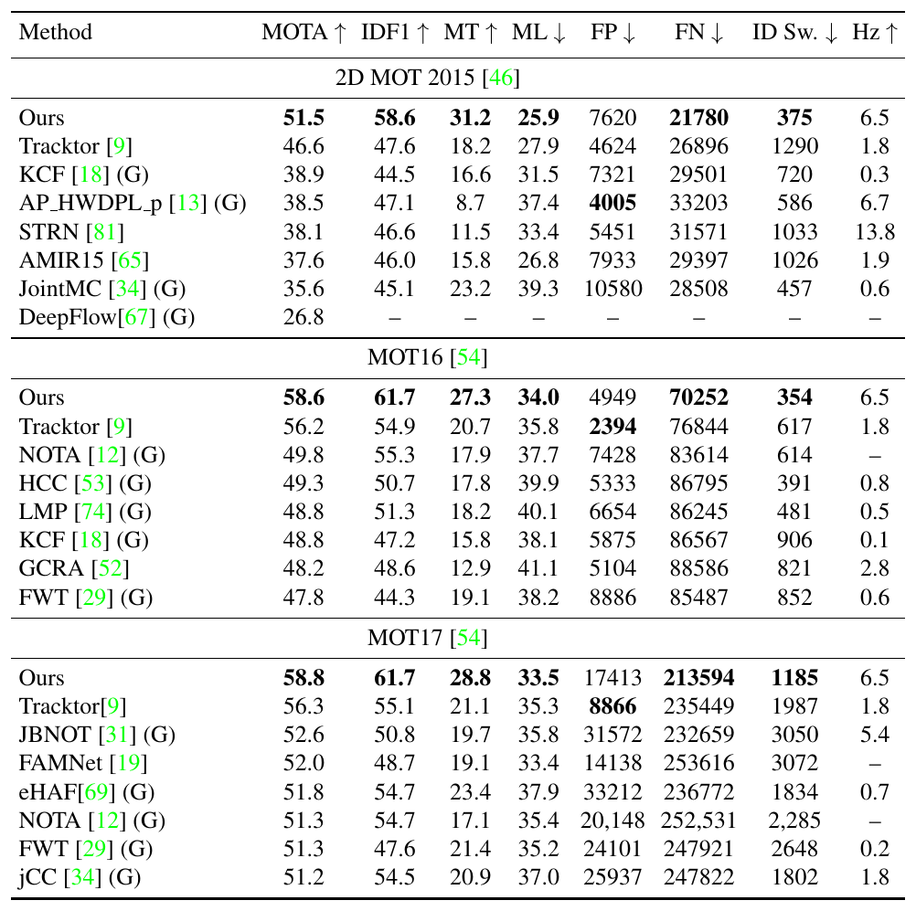
All three benchmarks use public detections. MPNTrack comes first on all three datasets, with IDF1 11, 6.4 and 6.6 points above the previous best results. Compared with other graph partitioning methods, it's not only much more accurate but also an order of magnitude faster than some of them; JointMC, for example, runs at only 0.6 Hz.
But Tracktor's preprocessing helps quite a bit here. In the appendix, the authors also report a version that drops Tracktor and instead corrects the public detections with a Faster R-CNN's regression head:
| Dataset | MOTA (with Tracktor) | MOTA (without) | IDF1 (with Tracktor) | IDF1 (without) |
|---|---|---|---|---|
| MOT15 | 51.5 | 46.6 | 58.6 | 53.8 |
| MOT16 | 58.6 | 54.3 | 61.7 | 56.8 |
| MOT17 | 58.8 | 56.0 | 61.7 | 58.4 |
Compiled from Table 7 in the paper's appendix.
Without Tracktor, MOTA drops by 2.8 to 4.9 points, and IDF1 by 3.3 to 4.9 points. Even so, it still beats the other graph methods in the table, and quite a few of those use raw detections without non-maximum suppression, low-level image features or hierarchical designs, so they have more information to work with than it does.
Limitations
MPNTrack is an offline method. Each graph needs to see future frames before it can make a decision, so it can't be moved straight into a real-time system.
The time window is short, too. A graph covers only about two seconds, so a person who is occluded for a long time won't be in the same graph when they walk back into view, and can't be linked back up. The number of edges grows with the square of the number of nodes, so a longer window would need much more aggressive pruning.
In 2023, the same lab's SUSHI stacked graphs into several levels, with lower levels handling short-term links and higher levels joining short tracks into long ones. The problem it tackles is exactly this window being too short.
Conclusion
Before this paper, learning in multi-object tracking was mainly used to learn features and costs, while what actually decided the tracks was still a traditional optimization solver. MPNTrack takes the binary variables of network flow directly as classification labels, uses message passing to let every edge see the whole graph, and lets the network learn near-feasible solutions by itself.
The time-aware update is an unassuming little change, just summing past and future separately, yet it lets the network learn the conservation constraints almost on its own.
The paper's title promises to learn a solver, and the network really did learn 98.8% of it. The remaining 1.2% still has to be handed to a rounding rule at the end, and a greedy loop is enough for that.