Original paper
Learnable Graph Matching: Incorporating Graph Partitioning with Deep Feature Learning for Multiple Object Tracking
- Publication
- CVPR 2021Conference
- First submitted to arXiv
- arXiv:2103.16178
Cite this paper · BibTeX
The citation identifies the linked source version. It cites the original paper and its authors.
@misc{multiobjecttrackinggmtracker2021,
  title = {{Learnable Graph Matching: Incorporating Graph Partitioning with Deep Feature Learning for Multiple Object Tracking}},
  author = {Jiawei He and Zehao Huang and Naiyan Wang and Zhaoxiang Zhang},
  year = {2021},
  eprint = {2103.16178},
  archivePrefix = {arXiv},
  url = {https://arxiv.org/abs/2103.16178}
}
From SORT to DeepSORT, most online trackers lay out the previous frame's tracks and this frame's detections as a bipartite graph, compute a similarity for every pair, and hand it to the Hungarian algorithm for matching.
This bipartite graph has only one kind of edge, "how similar track and detection are." How two detections in the same frame relate to each other, or which of two tracks was to the left of the other, is never taken into account.
Jiawei He and Zhaoxiang Zhang of the Institute of Automation, Chinese Academy of Sciences, and Zehao Huang and Naiyan Wang of TuSimple argue that these relations are the most reliable cue under occlusion. Pedestrians often walk in groups. When one person is blocked and their appearance is hard to make out, we can still recognize them again from "who they were walking next to."
Defining the problem
The authors identify three problems with data association at the time:
- Context within a frame is ignored. Whether it's bipartite matching between two frames or min-cost flow across many frames, only "cross-frame" matches count; the relations among objects within the same frame go unused.
- End-to-end methods rely on the network alone to fit. Some methods have the network output the matching directly, without using the tools that combinatorial optimization has built up over decades.
- The features for optimization methods are trained separately. In methods that do association with graph optimization, the features usually come from a separately trained network, so the training objective and the matching used at inference don't agree.
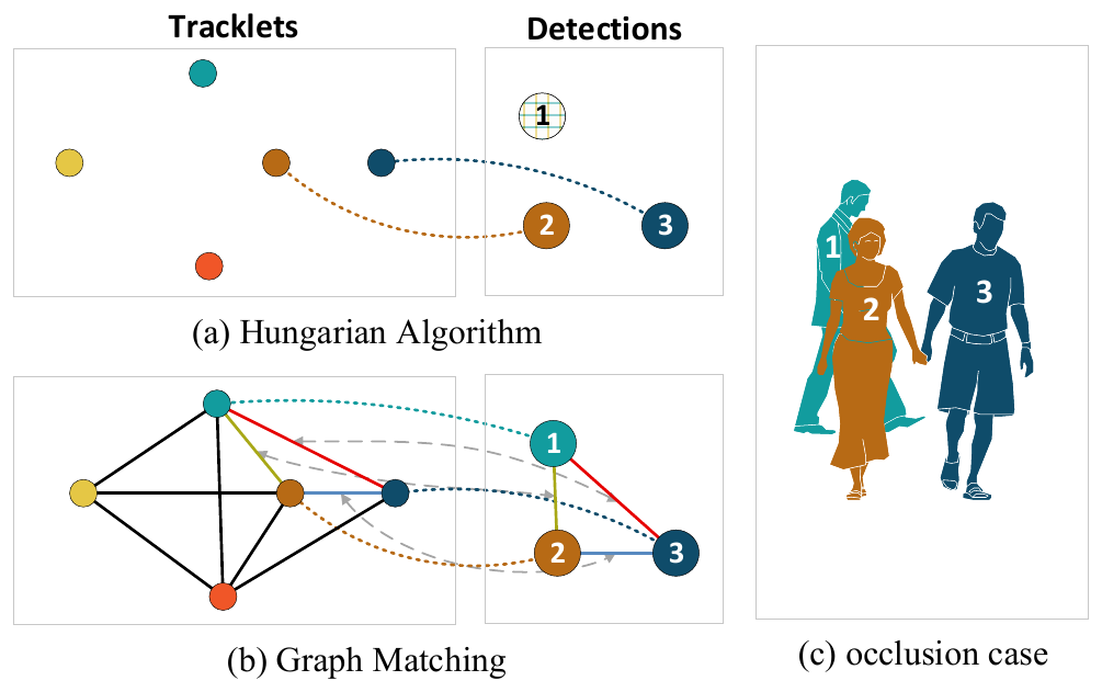
Look at (c) on the right. Number 1 is mostly hidden behind number 2, so the appearance feature extracted for them is probably unreliable. The Hungarian algorithm in (a) only asks "which track does this detection look like," so number 1 goes unmatched. (b) also looks at the relative positions among detections 1, 2 and 3, which line up with the relative positions among the tracks, and so number 1 is recognized again.
The authors call this "edge-to-edge" relation second-order similarity. Once it's used in association, the matching problem is no longer bipartite matching but general graph matching.
Solving the problem
From bipartite matching to graph matching
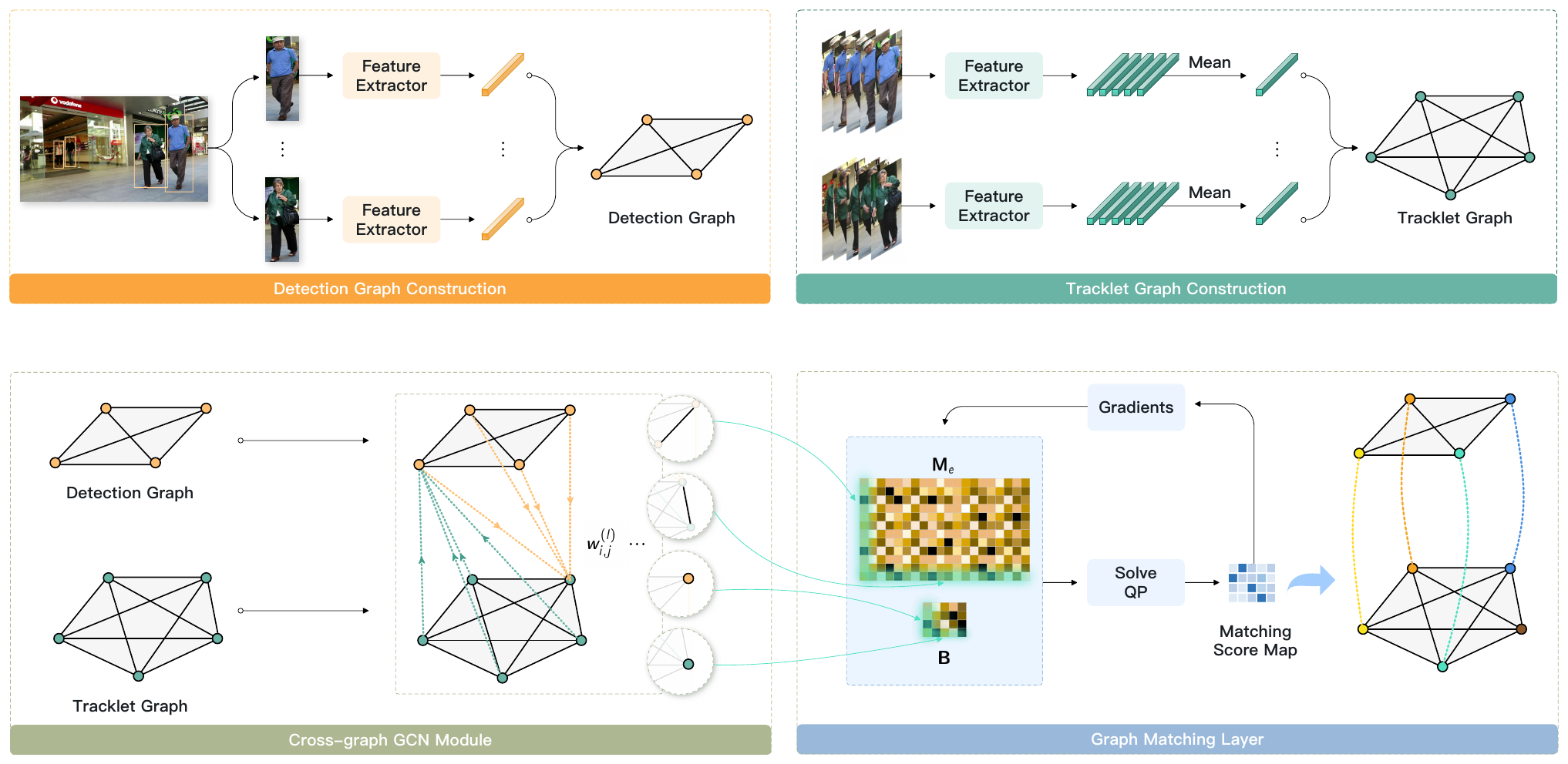
For each frame, the authors build two graphs. The vertices of the detection graph are this frame's detections, and the vertices of the track graph are the current tracks. Both are complete graphs, with an edge between every two vertices.
Graph matching looks for a matching under which matched vertices are similar to each other and matched edges are similar to each other too. Written mathematically, it's a quadratic assignment problem:
and are the edge weights of the two graphs, and is the similarity between vertices. The first term asks matched edges to have similar weights, and the second asks matched vertices to be similar.
The second term alone is the usual Hungarian algorithm. The first term is the new part.
An example with twins
Let's use an extreme example to see what the first term is good for.
Take two tracks, and , with always walking to the left of . This frame has two detections, and , but the two people are twins dressed identically, so every appearance similarity is 0.5.
Looking only at vertices, the two possible matchings score the same:
| Matching | Vertex score |
|---|---|
| –, – | 0.5 + 0.5 = 1.0 |
| –, – | 0.5 + 0.5 = 1.0 |
The Hungarian algorithm can only pick one at random.
Now add edges. GMTracker's edge feature concatenates the features of the two endpoint vertices, so edges have a direction; and are different edges. Suppose detection is to the left of . The similarity between edge and is 0.9, while with it's only 0.2; the same holds in the other direction.
| Matching | Vertex score | Edge score | Total |
|---|---|---|---|
| –, – | 1.0 | 0.9 + 0.9 | 2.8 |
| –, – | 1.0 | 0.2 + 0.2 | 1.4 |
Worked example for this note.
Two people you can't tell apart by looks alone can be told apart by where they stand relative to the people around them.
Relaxing into a differentiable quadratic program
The trouble is that the quadratic assignment problem is NP-hard. There's no polynomial-time algorithm for it like the Hungarian algorithm, let alone a way to put it inside a neural network and backpropagate through it.
The authors take two steps:
- Relaxation. The permutation matrix, whose entries can only be 0 or 1, is relaxed into a "doubly stochastic matrix" whose rows and columns each sum to 1. This is the tightest convex relaxation of permutation matrices, so the problem becomes a convex quadratic program.
- Edge features in place of edge weights. Instead of a single weight, each edge is now a vector. The similarity between two edges is the cosine similarity of their edge features; these form an edge-to-edge similarity matrix , which is then expanded into the matrix of the quadratic term.
The problem to solve in the end is:
is the matching matrix flattened into a vector, and is the vertex similarity. The constraints are that each detection's matching scores sum to 1 and each track's sum to at most 1, since some tracks have disappeared in this frame.
The optimal solution of a quadratic program can be differentiated with respect to its inputs using the KKT conditions and the implicit function theorem. Following OptNet, the authors turn the whole graph matching step into a differentiable network layer. During training, gradients pass through this layer back to the features; at inference only the forward solve is needed.
This solves the third problem above. The features are trained so that graph matching gets the matching right, and training and inference use the same matching method.
Cross-graph graph convolution
Vertex features come from a pretrained ReID network followed by two trainable fully connected layers. A track's feature is the average of all its detection features.
Before going into graph matching, the features are first enhanced by a layer of cross-graph graph convolution. Each vertex in the detection graph gathers messages from all the vertices of the track graph, weighted by appearance and position similarity:
A track's box is predicted by a constant-velocity Kalman filter. In videos where the camera moves, the predicted position is unreliable, so only appearance similarity is used.
The gathered message is normalized, added back to the original feature, and passed through an MLP:
The track graph's vertices are updated the same way. As in MPNTrack, messages pass only between the two graphs, not within either one. Finally, each edge's feature is the concatenation of its two endpoint features, l2-normalized.
Training and inference
Training uses a weighted binary cross-entropy, with positives weighted by to offset the imbalance of each detection having only one correct track but many wrong ones. The quadratic program's solution is fairly smooth, so before computing the loss, a softmax with a very low temperature () pulls the scores apart.
At inference, the relaxed solution isn't necessarily 0 or 1, so the authors round it greedily, assigning each detection to its highest-scoring track. Track creation and deletion follow DeepSORT. Detections whose appearance is too dissimilar, that are too far from every track (the Kalman filter's Mahalanobis distance exceeds a threshold), or that don't overlap any track sit out the matching at first; afterwards these detections are matched once more against the unmatched tracks using IoU and the Hungarian algorithm. ECC is also added for camera motion compensation. A track is deleted only after going 100 frames without an update.
Discussion
What each part contributes
The ablations use three-fold cross-validation on the MOT17 training set, with DeepSORT's Hungarian matching as the baseline:
| Setup | IDF1 | MOTA | ID switches |
|---|---|---|---|
| DeepSORT baseline | 68.1 | 62.1 | 1,135 |
| + graph matching | 70.0 | 62.3 | 1,128 |
| Full GMTracker | 71.5 | 62.3 | 1,017 |
| Perfect association | 77.2 | 62.6 | 14 |
Compiled from Table 1 and appendix Table A of the paper, MOT17 validation set, without interpolation.
- Graph matching itself contributes the most. Just swapping the Hungarian algorithm for graph matching adds 1.9 IDF1. The trained appearance features and graph convolution add about 0.6 more, and adding position information about 1.0 more.
- MOTA barely moves. From 62.1 to 62.3, because GMTracker deals with association and the detections don't change. That's also why the authors use IDF1 as the main metric.
- It's still some way from perfect. In the appendix, the authors do perfect association with the ground truth, and IDF1 is 77.2. GMTracker closes about a third of the gap between the baseline and perfect.
The graph matching layer only pays off when it's trained along with everything else. Used in neither training nor inference, IDF1 is 69.5; added only at inference, 70.2; only when used in both training and inference does it reach 71.5.
How long can it hold on?
| Frames kept | 30 | 50 | 80 | 100 | 150 |
|---|---|---|---|---|---|
| Hungarian | 67.2 | 67.9 | 68.1 | 68.1 | 67.3 |
| Graph matching | 68.0 | 69.3 | 69.7 | 70.0 | 70.0 |
Compiled from Table 4 of the paper, MOT17 validation set, IDF1.
The longer tracks are kept, the more candidate tracks there are, and at 150 frames the Hungarian algorithm actually drops 0.8, because more candidates make mismatches easier. Graph matching holds steady or rises all the way, and on that basis the authors conclude that GMTracker can match back tracks that have been gone for about 5 seconds.
With many candidates, comparing appearance alone makes it easy to mistake one person for another; bring in the relative relations as well, and a wrong combination is much harder to piece together.
Compared with other methods
On the MOT17 test set, with public detections refined by Tracktor, the online GMTracker gets an IDF1 of 63.8 and a MOTA of 56.2, higher than the other online methods of the time; with CenterTrack's detections, IDF1 is 66.9. With linear interpolation added to compare against offline methods, IDF1 is 65.9, above MPNTrack's 61.7 and LifT's 65.6; with CenterTrack detections plus interpolation, IDF1 is 68.7 and MOTA 65.0.
Mind the detection conditions in these comparisons. MOTA is driven mainly by detection, so for the very same GMTracker, switching to another set of detections makes MOTA jump from 56.2 to 61.5.
The cost
The paper doesn't report speed. The number of variables in the quadratic program is the number of detections times the number of tracks, and the edge-to-edge similarity matrix is much larger still; at inference the authors switch to CVXPY and do only the forward solve. In crowded scenes, a quadratic program has to be solved every frame, so the computational cost is something to assess before using it.
The later extended journal version applies the same learnable graph matching to image keypoint matching and point cloud registration, and its title changes to "A Practical Paradigm for Data Association."
Conclusion
GMTracker changes matching in online tracking from bipartite matching, which looks only at vertices, to graph matching, which looks at both vertices and edges. When a person is blocked and their appearance is unreliable, their position relative to the people around them can still identify them again. To fit this inside a neural network, the authors relax the quadratic assignment problem into a convex quadratic program and compute gradients through the KKT conditions, so the features are learned for the sake of matching.
This paper and MPNTrack both treat the relations among objects as cues for association, going beyond pairwise comparison. MPNTrack has a graph network predict directly which edges to connect, while GMTracker keeps the optimization solver and has the network learn only the features.
SUSHI, also from the MPNTrack team, later pushed the graph network approach to long-term tracking.
Reference
- Learnable Graph Matching: A Practical Paradigm for Data Association (extended TPAMI 2024 version)