Original paper
Towards Real-Time Multi-Object Tracking
- Publication
- ECCV 2020Conference
- First submitted to arXiv
- arXiv:1909.12605
Cite this paper · BibTeX
The citation identifies the linked source version. It cites the original paper and its authors.
@misc{multiobjecttrackingjde2019,
  title = {{Towards Real-Time Multi-Object Tracking}},
  author = {Zhongdao Wang and Liang Zheng and Yixuan Liu and Yali Li and Shengjin Wang},
  year = {2019},
  eprint = {1909.12605},
  archivePrefix = {arXiv},
  url = {https://arxiv.org/abs/1909.12605}
}
Trackers of the DeepSORT, POI and MOTDT generation all work in much the same way. First run a detector, then crop out every detection box and send it through a separate re-ID network to extract appearance features.
Each of the two networks runs once, so the time is the two added together. The more people in the frame, the more re-ID passes there are to run, and the slower the whole system gets.
Plenty of papers call themselves "real-time tracking," but look closely and the timing often covers only the association step, without the time for the detector and re-ID. The association is real time; the tracking system as a whole isn't.
Zhongdao Wang of Tsinghua University, Liang Zheng of the Australian National University and colleagues wanted to build a system that's truly real time. They had the detector recognize people while it was at it: the same network, in a single forward pass, outputs both the detection boxes and an appearance feature for each box. They call this approach JDE (Joint Detection and Embedding).
Defining the problem
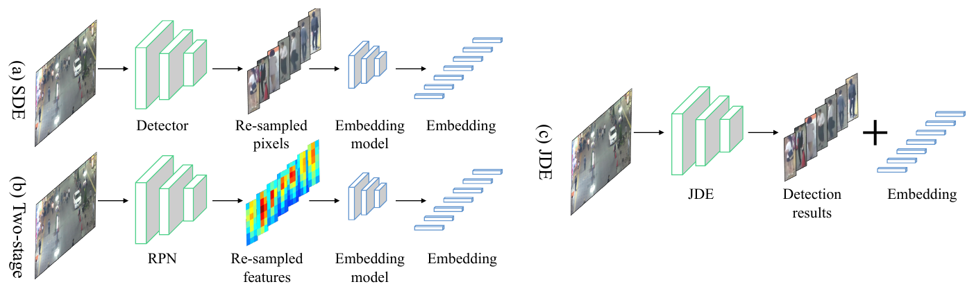
The authors divide the approaches of the time into three kinds:
- (a) Separate Detection and Embedding (SDE): DeepSORT and POI both belong here. The detector and the re-ID model are completely independent, and the amount of re-ID computation is proportional to the number of people.
- (b) Two-stage models: these take Faster R-CNN and turn its second stage into one that learns appearance features. The first-stage RPN outputs boxes as usual, and the second stage pulls each box's features from the feature map and trains them with metric learning instead. This shares part of the computation, but the two-stage design is slow in itself, usually under 10 frames per second, and the second stage's time still grows with the number of people.
- (c) JDE: add one more output directly onto a single-stage detector, so that a single forward pass gives both boxes and features.
Getting to (c) means having two tasks with very different objectives learn well together in the same network. The authors work through this from five angles, one by one: training data, network architecture, loss functions, multi-task weighting and evaluation.
Solving the problem
Network architecture

The backbone is DarkNet-53, as used in YOLOv3, with a feature pyramid network (FPN) on top, predicting at three scales: 1/32, 1/16 and 1/8 of the input. Pedestrians vary a lot in size depending on how far away they are, and multi-scale prediction helps detection.
Each scale gets a prediction head that outputs a dense prediction map of size . is the number of anchor boxes at this scale, and is the dimension of the embedding. The map is split into three parts:
- Box classification: , whether each anchor box is foreground or background.
- Box regression: , four offsets for each anchor box.
- Embedding map: , a -dimensional appearance feature at each position.
Let's work out the shapes for the default input of . The feature maps at the three scales are , and . The paper doesn't give the value of ; in FairMOT's experiments, JDE uses 512 dimensions. Each scale has , so each prediction head outputs channels, and the finest layer is a tensor.
When an anchor box is judged to be foreground, the 512-dimensional vector at the same position in the embedding map is taken as that box's appearance feature. Detection and appearance features are computed together, so one more person in the frame barely changes the amount of computation.
The detection branch: anchors tuned for pedestrians
The detection branch is broadly the same as an RPN, with two modifications:
- Anchors designed specifically for pedestrians. Every anchor has an aspect ratio of 1:3, with 12 sizes in total, 4 per scale, and widths running from all the way to pixels.
- Foreground and background thresholds. An IoU above 0.5 with a ground-truth box counts as foreground, the same as in ordinary object detection; but an IoU below 0.4 (instead of the usual 0.3) already counts as background. The authors found this effectively suppresses false positives under heavy occlusion.
Classification uses cross-entropy, and box regression uses smooth-L1.
The embedding branch: classification instead of triplets
The embedding has to learn a space where features of the same person sit close together and features of different people are far apart. The most intuitive approach is a triplet loss, which is how MOTDT was trained. But there are too many possible triplets, sampling is hard, training tends to be unstable and convergence is slow.
The authors compare three losses:
- Triplet loss: within a mini-batch, mine all the negatives and the hardest positive.
- Smooth upper bound of the triplet loss: a variant that's more stable and converges faster.
- Cross-entropy: treat every identity in the training set as a class, pass the extracted embedding through one fully connected layer, and classify identities.
The authors first compare the last two in their formulas. The smooth upper bound can be written as
and the cross-entropy as
The two look almost identical, with two differences. First, cross-entropy represents each identity with a learnable "class weight" , instead of using the features of other samples directly. Second, the cross-entropy denominator includes all other identities, while the triplet-style losses include only the negatives drawn in this mini-batch. Cross-entropy requires a person to be closer to their own class than to every other identity, a much stricter constraint than the triplet one.
The experimental results are lopsided too. Under the same weighting settings, the embedding's TPR@FAR=0.1 on the retrieval task is only 42.2 for the triplet loss and 44.3 for the smooth upper bound, against 88.2 for cross-entropy, a full doubling.
Foreground anchors that have a box but no identity label are ignored when computing the embedding loss. The embeddings from all three scales go through the same fully connected layer and share one feature space, so the same person detected at different scales can still be compared.
Balancing the three losses
Each prediction head has three losses, which makes nine across the three scales. The simplest approach is to add them all up with equal weights, but that barely trains at all.
The authors compare several weighting strategies:
- Uniform: detection AP drops to just 6.8. The embedding loss is much larger in magnitude than the other two, so it dominates training, detection never gets learned properly, and MOTA is only 36.9.
- MGDA-UB: the most theoretically sound multi-task optimization method, but it gives the embedding loss too much weight, and the result is about the same as uniform weighting, with an AP of 8.3.
- Loss normalization (Loss.Norm): uses the reciprocal of each loss's moving average as its weight; MOTA 57.9.
- Approximate optimal weights (App.Opt): constrained to two independent variables, with a set of weights found by manual search; MOTA 64.3.
- Uncertainty weighting (Uncertainty): each loss gets a learnable parameter , and the network decides the weights for itself:
This last method is the only one that beats the manual search, with an AP of 83.0, a TPR of 90.4 and a MOTA of 65.8, and its 207 ID switches are also the fewest. FairMOT adopted the same weighting scheme the following year.
Training data
JDE needs data that has both box and identity annotations, but tracking datasets are too small. The authors stitch six public datasets into one large training set. ETH and CityPersons have boxes only, so they train only detection; CalTech, MOT16, CUHK-SYSU and PRW have identity annotations, so both branches train on them. In total there are about 54,000 images, 270,000 boxes and 8,700 identities. Videos in ETH that overlap with the MOT16 test set have been removed.
FairMOT later called this combination MIX, and it became the standard training data for one-shot trackers.
Association
Association isn't the focus of this paper; the authors designed a simple, fast online association. Each track keeps an appearance state and a Kalman filter motion state. Every frame, the appearance similarity (cosine similarity) and the motion distance (Mahalanobis distance) between all detections and tracks are computed and weighted into a cost:
After matching with the Hungarian algorithm, a track's appearance state is updated with an exponential moving average:
Only a detection that shows up in two consecutive frames starts a new track; a track is deleted only after 30 frames without an update, and in between it stays in a holding pool, so it can still be picked up again when it comes back.
StrongSORT and BoT-SORT later borrowed this EMA update directly. The authors also mention that vectorizing the Kalman filter (handling all tracks at once) is crucial for speed: once the network is already fast, association can easily become the bottleneck.
Discussion
JDE is trained with SGD for 30 epochs, with a default input resolution of . For validation, detection is measured by AP on the CalTech validation set, embedding by retrieval TPR on three datasets, and tracking by MOTA on the MOT15 training set; the final comparison is on the MOT16 test set.
Association methods
The authors first attach the same JDE model to SORT and to their own association method. On MOT15, with few people, their method gets a MOTA of 67.5 and an IDF1 of 67.6, against SORT's 66.9 and 55.8, and speed also goes from 44.1 to 46.2 FPS. On the crowded CVPR19-01 sequence (61 people per frame on average), speed goes from 26.4 to 33.9 FPS, while MOTA and IDF1 improve only slightly. The big improvement in IDF1 comes mainly from the appearance features.
Compared with separate systems
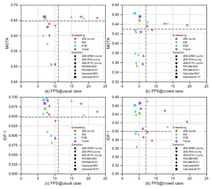
For a fair comparison, the authors use exactly the same training data, pair up several detectors (JDE, Faster R-CNN, Cascade R-CNN) with several re-ID models (IDE, Triplet, PCB), and attach the same association to each.
- The best trade-off between speed and accuracy. With few people, JDE runs at 22 frames per second with a MOTA of 65.8; the strongest combination, Cascade R-CNN (ResNet-101) plus PCB, gets a MOTA of 66.2 but runs at only about 6 frames per second.
- The gap widens in crowds. Every SDE combination slows down sharply in crowded scenes, because re-ID time is proportional to the number of people; JDE computes its embeddings together with detection, so its speed is barely affected, and what slowdown there is comes mainly from association.
- Jointly learned embeddings are as good as separately learned ones. Keeping JDE's detector fixed and swapping in independently trained IDE, Triplet and PCB embeddings gives very similar tracking accuracy, and JDE even edges out IDE.
The IDF1 side isn't so pretty, though. In crowded scenes, JDE's IDF1 drops more than that of the strong SDE combinations.
The MOT16 test set
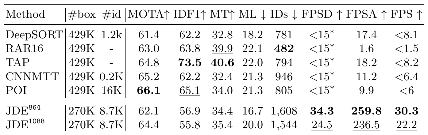
JDE uses extra training data, so it's compared under MOT16's private protocol. Its competitors all use the same Faster R-CNN trained on large private pedestrian data, and differ in their re-ID models and association methods.
On MOTA, JDE's 64.4 is 3 points above DeepSORT and 1.7 points below POI, while it trains on only a little over 60% as many boxes as its competitors (270,000 vs. 429,000). On speed, many methods don't report the full time, so the authors reimplemented the detector they share to estimate an upper bound; even against such a generous upper bound, JDE at 22.2 frames per second is at least two to three times faster. Shrinking the input width to 864 raises the speed to 30.3 FPS, while MOTA drops only to 62.1.
But IDF1 and ID switches are JDE's clear weak spots. Its IDF1 of 55.8 is lower than DeepSORT's 62.2 and POI's 65.1; its 1,544 ID switches are nearly twice those of the other methods.
The boxes are the problem
At first the authors suspected the jointly learned embedding was weaker. But after swapping the embedding for independently trained models, IDF1 and ID switches barely changed.
The real cause is detection. When pedestrians overlap heavily, the single-stage detector's boxes tend to drift and misalign, and when features are taken from misaligned boxes, they pick up parts of other people, so IDs switch along with them. These ID switches often happen in the middle of a track, which is why IDF1 drops so much. The authors leave "how to make boxes more accurate when pedestrians overlap heavily" to future research.
What came after
Someone took up this problem just half a year later. FairMOT argues that the anchors are to blame. One anchor box may cover several people, and several anchor boxes may correspond to the same person, so the re-ID features come out muddled. FairMOT switches to an anchor-free center-point representation and cuts the embedding down to 64 or 128 dimensions. In FairMOT's experiments, simply reducing JDE's embedding from 512 to 64 dimensions improved MOTA, IDF1 and ID switches across the board.
Conclusion
JDE packs appearance features into a single-stage detector and outputs boxes and features in one forward pass, making it the first complete multi-object tracking system to come close to real time. Its MOTA on MOT16 is close to that of strong separately trained systems, it's two to three times faster, and the more people there are, the bigger its advantage.
The two training details are what's most worth taking away from this paper. Using identity-classification cross-entropy for the embedding is twice as good as a triplet loss, and letting uncertainty parameters learn the multi-task weights beats manual search. Both tricks became more or less standard in later one-shot trackers.
The paper's title says "Towards," and the authors knew full well that the stretch of road where boxes don't line up would have to be left for the next paper to walk.