Original paper
Simple Online and Realtime Tracking with a Deep Association Metric
- Publication
- ICIP 2017Conference
- First submitted to arXiv
- arXiv:1703.07402
Cite this paper · BibTeX
The citation identifies the linked source version. It cites the original paper and its authors.
@misc{multiobjecttrackingdeepsort2017,
  title = {{Simple Online and Realtime Tracking with a Deep Association Metric}},
  author = {Nicolai Wojke and Alex Bewley and Dietrich Paulus},
  year = {2017},
  eprint = {1703.07402},
  archivePrefix = {arXiv},
  url = {https://arxiv.org/abs/1703.07402}
}
SORT stripped the tracker down to a Kalman filter, IoU and the Hungarian algorithm. It was blazingly fast, and its MOTA wasn't bad either. But its ID switch count always looked ugly.
The reason isn't hard to guess. SORT knows only a box's position and size. If an object is occluded for two frames, its track gets deleted; when it reappears, the tracker has no clue that "I saw this person a moment ago," so it hands out a new ID.
A year later, SORT's author Alex Bewley teamed up with Nicolai Wojke and Dietrich Paulus of the University of Koblenz-Landau in Germany to fill this gap. Their fix is simply to make the tracker remember what each person looks like.
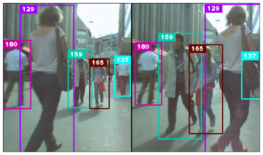
This is DeepSORT's output on MOT16. Between the two images, people cross paths. 129 in the foreground walks from the middle of the frame to the right and blocks 137 behind them; 159 and 165 in the distance come closer, and their boxes grow several times larger. None of the five IDs changes.
The paper is only five pages long, yet it became the most widely used tracker for years afterwards, and the "Deep" in its name is often misunderstood. Let's take it slowly.
Defining the problem
The authors start by tracing SORT's ID switches to their cause. SORT matches on the IoU between predicted boxes and detection boxes, and that measure is only reliable when the state estimate is accurate.
Once an object is occluded, the Kalman filter can only keep predicting, with no updates. The predicted box drifts further and further away and no longer overlaps the detection box when the object reappears. In frontal-view street scenes, pedestrians occluding one another is the norm, so SORT keeps breaking tracks and reissuing IDs.
Solving this takes a cue that still works when position can't be trusted. The authors chose appearance. They use a convolutional network trained on a large person re-identification (re-ID) dataset to turn every detection box into a feature vector. Features of the same person at different times should be close; features of different people should be far apart.
The design keeps SORT's spirit by pushing the complex parts into an offline stage. The network is trained in advance, and online tracking does only nearest-neighbor lookups, with no online learning at all.
Solving the problem
State and track management
The Kalman filter framework largely follows SORT, but the state becomes eight-dimensional:
is the box center, the aspect ratio, the height, and the last four entries are the corresponding velocities. Compared with SORT, area has been replaced by height, and the aspect ratio now has its own velocity. A detection box's is used directly as the observation.
Each track keeps a counter of how many frames have passed since its last successful match. It goes up by one at every prediction and resets to zero on a successful match. Once it exceeds the limit , the object is considered to have left the scene, and the track is deleted.
A new track's first three frames are a probation period (tentative). It has to be matched successfully in every one of those three frames, or it's deleted on the spot; only after surviving all three does it switch to the confirmed state.
SORT's is 1; here, is set to 30 in the experiments. A track can survive a full second of absence, provided it's recognized when it comes back.
Two distances
Matching is still an assignment problem, but the cost matrix becomes a combination of two distances.
The first is the Mahalanobis distance, which describes motion:
are the mean and covariance of the -th track's predicted distribution projected into observation space, and is the -th detection box. Unlike IoU, the Mahalanobis distance factors in uncertainty: it measures how many "standard deviations" the detection box is from the predicted center.
This distance can be used to rule out impossible matches. The observation space is four-dimensional, so the squared Mahalanobis distance follows a chi-square distribution with 4 degrees of freedom. Taking the 95% confidence interval gives the threshold , and anything beyond it isn't allowed to match.
The second is the appearance distance. Each detection box goes through the network to get a unit-length feature , and each track keeps the features from its last 100 successful matches as a gallery . The appearance distance is the cosine distance between the detection's feature and the most similar one in the gallery:
The advantage of taking the minimum is that when a person turns around or walks into shadow, they can still be recognized, as long as the gallery holds a feature from a similar angle. The appearance distance also has its own threshold , set on separate training data; the official code defaults to 0.2.
The two combine into the final cost:
and a match is admissible only if it passes both thresholds.
The authors are clear about how the two divide the work. The Mahalanobis distance suits short-term prediction and is most useful when an object has just been seen and its position is certain. The appearance distance suits recovering identities after long occlusions, when motion information no longer has much discriminative power.
Then comes a detail that often gets overlooked. In their experiments, the authors set to 0.
In other words, only the appearance distance is left in the cost matrix, and the Mahalanobis distance only acts as a gate, blocking matches that are impossible given the positions. The authors' reasoning is that when the camera moves noticeably, displacements in the image plane vary a lot, and the Kalman filter's prediction is only a rough estimate. Many tutorials describe DeepSORT as "a weighted sum of position and appearance," but the paper's actual results come from "appearance ranks, motion gates."
The matching cascade
Instead of throwing all the tracks and detection boxes into a single assignment problem, the authors designed a matching cascade.
Why do this? The problem lies in the Mahalanobis distance itself. Let's work through it once in one dimension (the numbers are made up for illustration).
Suppose track A was seen just last frame, with a predicted position of 100 and a standard deviation of 5. Track B has been occluded for a dozen or so frames, with a predicted position of 120, but because it hasn't been updated all that time, its standard deviation has ballooned to 30. Now a detection box shows up at 108.
- For A, the detection box is off by 8, which is standard deviations, a squared Mahalanobis distance of 2.56.
- For B, the detection box is off by 12, only standard deviations, a squared Mahalanobis distance of 0.16.
A, which is closer and whose state is more certain, ends up losing.
Intuitively, the longer a track has gone unseen, the less sure we should be that it has anything to do with any detection box, so its distance ought to grow. But the Mahalanobis distance uses the standard deviation as its unit, so the greater the uncertainty, the "closer" every detection box looks. When two tracks compete for the same box, it favors the more uncertain one.
The cascade handles this by processing tracks in tiers, by "how long since last seen":
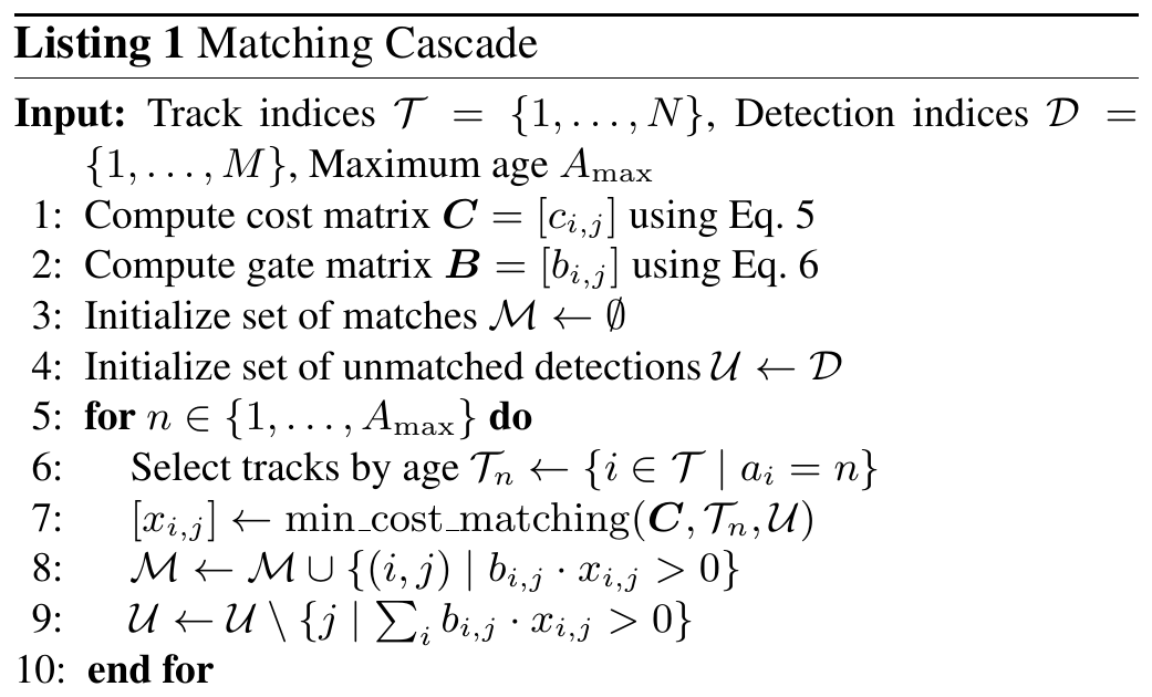
The loop on line 5 starts at , handling the tracks that were matched just last frame first and letting them pick detection boxes; the remaining detection boxes then go to the tracks, and so on, up to . In the example above, A takes the detection box in the very first tier, and B never gets a turn.
After the cascade there's one last step. Tracks still on probation, and tracks of age that didn't get matched, go through one round of SORT-style IoU matching against the remaining detection boxes. This step handles sudden changes in appearance, such as being half hidden behind a static object, and it also gives newly created tracks, whose appearance galleries are still small, a chance to carry on.
The appearance network
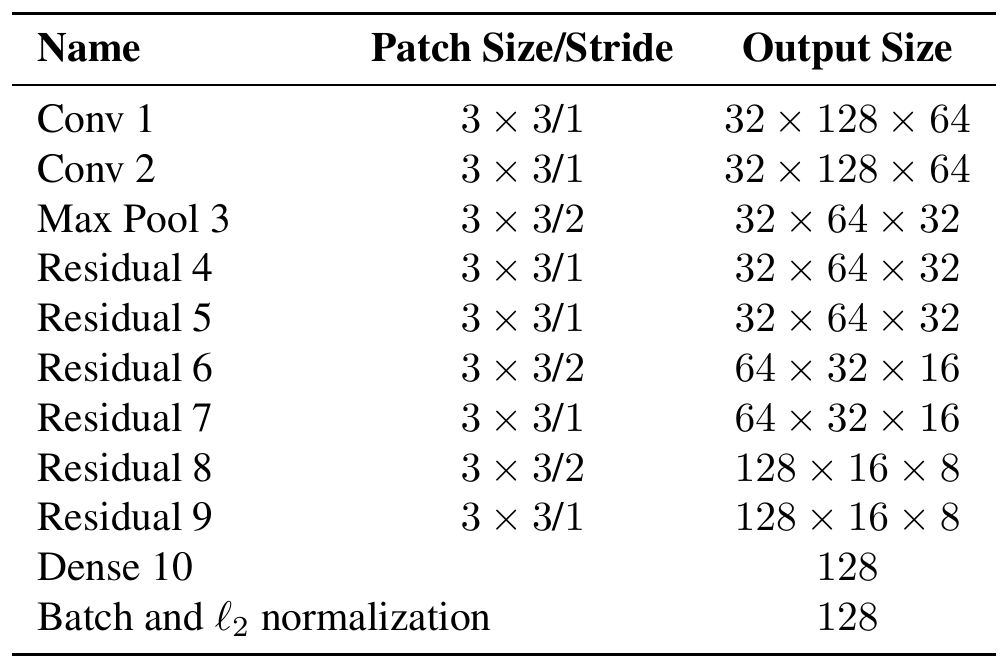
The network is a wide residual network with two convolutional layers, six residual blocks and a final fully connected layer that outputs 128 dimensions. The batch normalization and L2 normalization at the end project the features onto the unit sphere, so the inner product of two features is their cosine similarity, which matches the appearance distance above.
The whole network has about 2.8 million parameters, and on a GTX 1050 laptop GPU, a batch of 32 boxes takes about 30 milliseconds. The training data is the MARS person re-identification dataset, with over 1.1 million images of 1,261 people.
The paper doesn't give the training details; the authors say they're out of scope. The official code's README points to the cosine metric learning method from another paper of theirs the following year.
Discussion
The authors evaluate on the MOT16 test set. MOT16 has seven test videos, including frontal-view street scenes from moving cameras as well as top-down surveillance footage.
The detections are the Faster R-CNN detections released by Yu et al. (the authors of the POI method), trained on public and private data and far better in quality than the official public detections. For a fair comparison, the authors reran SORT with the same detections. The settings are , and a detection confidence threshold of 0.3.
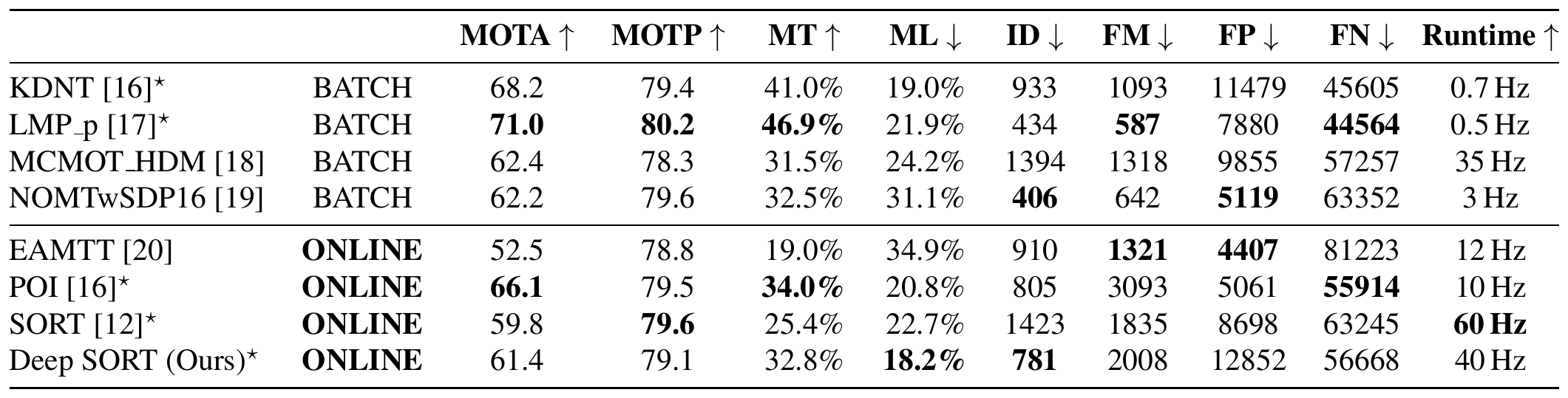
In this table, the methods marked with an asterisk all use the same POI detections. Let's compare the SORT and Deep SORT rows first, since they're the only two whose difference comes purely from the tracker:
- ID switches drop from 1423 to 781, about 45% fewer. This is the main payoff of adding appearance, and it's also the fewest in the online group.
- MT rises from 25.4% to 32.8%, and ML falls from 22.7% to 18.2%. Identities are held for longer, so more trajectories are tracked most of the time, and fewer are almost completely lost.
- FM rises from 1835 to 2008. The authors explain that tracks now survive occlusions and missed detections, so the empty frames in the middle count as one fragmentation.
- FP rises from 8698 to 12852. This is the main reason MOTA only goes from 59.8 to 61.4.
That last point deserves a second look. Inspecting the output, the authors found that most of the extra false positives come from the detector's occasional misfires on static background. keeps tracks alive for a long time, so these sporadic false positives get stitched into tracks, forming stable fake tracks that sit motionless in one place. The authors also observed that tracks rarely jump between false positives. In other words, these false positives mainly drag down MOTA and do little harm to identity preservation. Raising the detection threshold could improve MOTA considerably, but the paper doesn't report that result.
Compared with the POI method, which uses the same POI detections, Deep SORT's MOTA is nearly 5 points lower, its ID switches slightly fewer (781 vs. 805), and its speed several times faster.
As for speed, the table lists 40 Hz; in the text, the authors say the full implementation runs at about 20 Hz, with nearly half the time spent generating appearance features. Neither number includes the detector itself.
What came after
DeepSORT's code is simple and its feature network can be swapped out directly, so it quickly became standard equipment in engineering projects. MATLAB has an official example of it, and the "YOLO + DeepSORT" combo projects on GitHub are too many to count.
Five years later, StrongSORT took it as the starting point for a renovation, replacing the appearance network and the Kalman filter, and also removing the matching cascade in favor of a single global assignment. Their ablation found that the cascade helps weaker trackers by cutting down on wrong matches, but once the tracker gets stronger, it ties the tracker's hands. In StrongSORT's table, switching the original DeepSORT to ordinary matching drops IDF1 by 1.1; as the tracker is progressively strengthened, the benefit of dropping the cascade becomes more and more apparent, and the two strongest versions gain 1.8 and 1.4.
None of this overturns DeepSORT's design. It just shows that the problem the cascade handles (uncertain tracks getting an edge in Mahalanobis distance) is less serious once the appearance features are strong enough and the cost matrix is no longer dominated by Mahalanobis distance.
Conclusion
An appearance network trained offline, plus a matching cascade that works through tracks in tiers by age, cut ID switches on MOT16 by 45%. Tracks can survive a full second of absence, and tracking itself still runs at dozens of frames per second.
Its "Deep" applies only to the appearance features. The motion model, the matching and the track management are all still hand-written rules, so swapping in a better re-ID network is usually the cheapest upgrade.
Oh, and when you use DeepSORT to track something other than pedestrians, remember to swap out that feature network trained on MARS. It knows a thousand-odd pedestrians, but it doesn't know your truck.