Original paper
Real-time Multiple People Tracking with Deeply Learned Candidate Selection and Person Re-Identification
- Publication
- ICME 2018Conference
- First submitted to arXiv
- arXiv:1809.04427
Cite this paper · BibTeX
The citation identifies the linked source version. It cites the original paper and its authors.
@misc{multiobjecttrackingmotdt2018,
  title = {{Real-time Multiple People Tracking with Deeply Learned Candidate Selection and Person Re-Identification}},
  author = {Long Chen and Haizhou Ai and Zijie Zhuang and Chong Shang},
  year = {2018},
  eprint = {1809.04427},
  archivePrefix = {arXiv},
  url = {https://arxiv.org/abs/1809.04427}
}
If you've read the code of FairMOT or JDE, there's a good chance you've seen the name MOTDT in the association part.
The FairMOT paper is direct about it, writing "We follow MOTDT (Chen et al., 2018a) and use a hierarchical online data association method." Of the three classic association methods ByteTrack compares against, two are SORT and DeepSORT, and the third is MOTDT.
The name turns up in other people's tables all the time, yet the paper itself is only six pages long. Long Chen, Haizhou Ai and colleagues at Tsinghua University published it in 2018, and it deals with a problem every tracker runs into: what to do when the detector can't be relied on.
Defining the problem
In crowded scenes, detectors make mistakes easily. A change in pose or being blocked by someone else, and you get missed detections, false positives or boxes in the wrong place.
Offline (batch) methods can look at the whole video and use future frames to correct these errors, but they aren't real time and can't be used in applications that need results on the spot. This paper does online tracking only, using just the current and past frames.
In traditional tracking-by-detection, the only candidate boxes during association are the detections. If the detector misses someone, there's no box at all in that frame to give to their track.
The authors noticed that detection and tracking can actually complement each other:
- Track predictions can cover short-lived missed detections or inaccurate boxes. If the detector doesn't find the person in this frame, the Kalman filter's predicted box is still there.
- High-confidence detections can keep tracks from drifting onto the background over the long run. A predicted box that never gets corrected by a detection will go astray sooner or later.
So why not treat both as candidates? But detection boxes and predicted boxes come from different sources. How do you score them with the same yardstick, and then pick the best out of a pile of overlapping boxes?
Earlier, Yan et al. had also tried treating the outputs of both the detector and the tracker as candidates, but with hand-crafted features such as color histograms and optical flow. This paper wants to do it with deep networks, and in real time.
Solving the problem
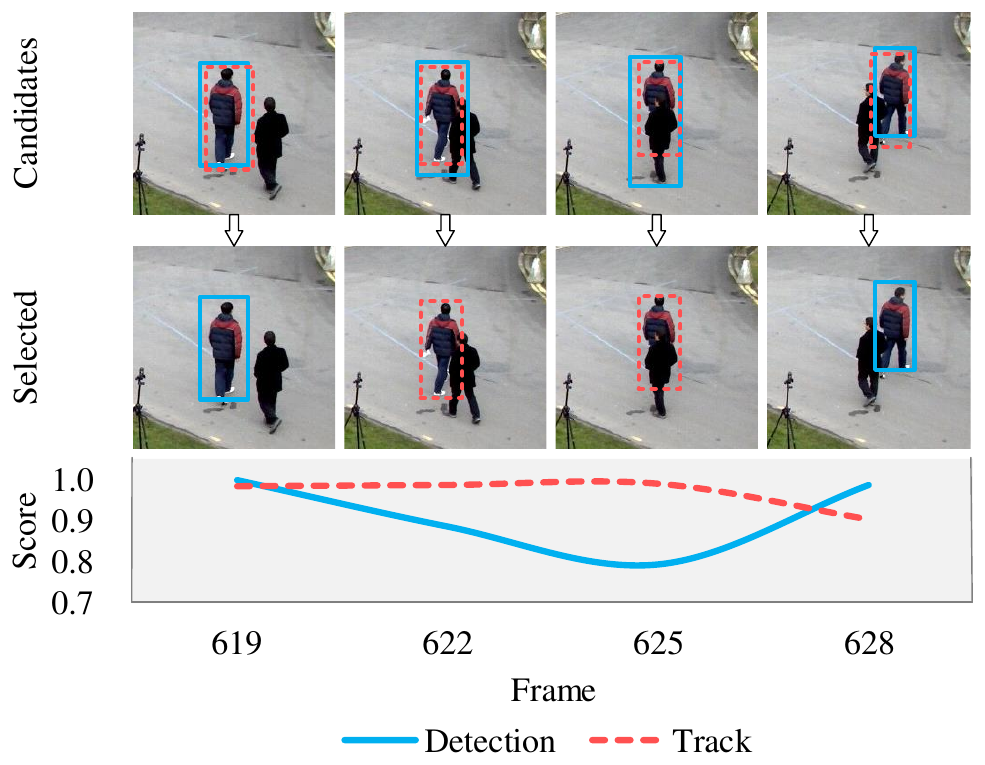
This figure is the whole idea of the paper. The solid blue lines are detection boxes, the dashed red lines are the track's predicted boxes, and the curves below are the scores of the two.
In the frames before and after, the detection box scores higher and gets selected. In between, from frame 622 to 625, the person is partly occluded, the detection box's score drops, and the predicted box becomes the more reliable one, so the selection switches to the predicted box.
The method has two steps: first select candidates, then associate.
1. One classifier scores every candidate
Detection boxes plus predicted boxes add up to a lot of boxes, and they overlap heavily. Cropping each box and sending it through a classification network would be too slow.
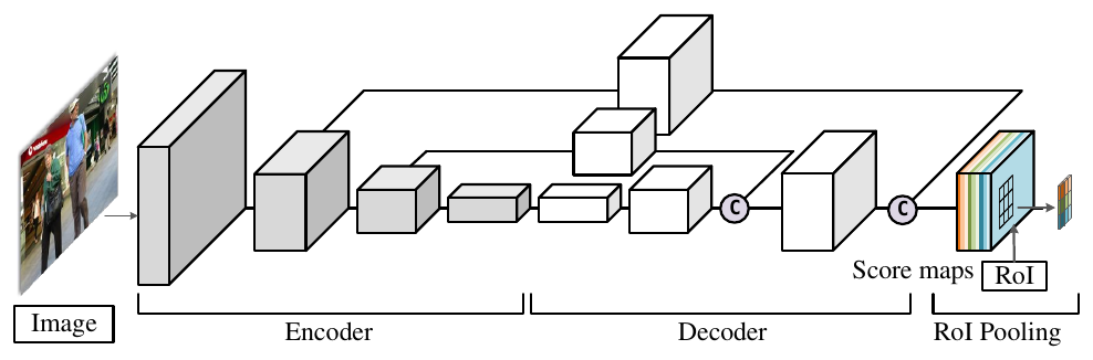
The authors switch to the R-FCN (region-based fully convolutional network) approach: the network runs only once over the whole image and outputs a few score maps, which all the candidate boxes share.
The backbone uses the lightweight SqueezeNet as its encoder, followed by a decoder with upsampling that raises the resolution of the score maps. For a input image, it takes only 8 milliseconds on a GTX 1080 Ti.
The simplest way to score would be to compute, at every point in the image, the probability that it's "person," and then average all the points inside the box. But that throws away spatial information. If a box covers only half a person, the points inside it are still all on the person, so the average still comes out high.
R-FCN solves this with position-sensitive score maps. The network outputs score maps, each candidate box is divided into a grid, and each cell reads only the score map that "belongs to its own position." Finally, the responses of the cells are averaged and passed through a sigmoid:
Picture it with . The network outputs 9 score maps, which respond to "a person's top-left corner," "a person's top center" ... "a person's bottom-right corner." When a box frames a person exactly, the top-left cell reads the top-left map, the bottom-right cell reads the bottom-right map, and every cell reads a high score. If the box is shifted half a person to the right, its right half lands on the background, the three cells on the right all read low scores, and the average drops.
This network only classifies; it doesn't regress boxes. In the implementation, . The training data consists of positive samples randomly drawn around ground-truth boxes and an equal number of background negatives, taken from MS COCO and two MOT16 training videos.
2. Track confidence: how long can a predicted box be trusted?
Predicted boxes are useful for a short while, but over time they become unreliable. The longer the Kalman filter goes without a detection to update it, the less accurate its prediction.
The authors define a confidence score for each track. A track may break off and be recovered several times, and every recovery reinitializes the Kalman filter, so only the last continuous tracklet is considered:
is the number of detections this tracklet has been matched to, and is the number of consecutive predictions used since the last time it was matched to a detection.
The formula behaves intuitively:
- Right after a detection is matched, and the confidence is 1.
- Each additional prediction adds one to , and the confidence falls logarithmically.
- Once exceeds , the confidence hits zero, and this track's predicted box can no longer be a candidate.
- A track has to be matched to at least two detections before there are enough observations to build a motion model, and only then can its predicted box be a candidate.
3. A unified score
The scores of the two kinds of candidates are defined as:
A detection box's score is simply the classification probability; a predicted box's score is the classification probability multiplied by the track confidence. Even if a predicted box looks very much like a person, its score gets pushed down if it comes from a track that hasn't been confirmed by a detection for a long time.
Once every candidate has been scored, non-maximum suppression is applied once (IoU threshold 0.3), and boxes scoring below 0.4 are discarded.
4. Appearance features
During association, deciding whether a candidate box and a track are the same person relies on re-ID features. The network uses the part-aligned architecture proposed by Zhao et al., with a GoogLeNet convolutional backbone followed by fully connected branches, each corresponding to a different body part. It outputs a 512-dimensional feature, compared by Euclidean distance.
The training data combines three person re-identification datasets, Market-1501, CUHK01 and CUHK03, and the network is trained with a triplet loss:
is the same person, and are different people. Triplets that are already well separated () have zero loss, so training concentrates on the hard examples.
5. Hierarchical association
This is the part that JDE and FairMOT later adopted. Association happens in two tiers:
- Tier one: detection candidates × tracks, by appearance. The distance between re-ID features is computed, with a threshold of 0.4.
- Tier two: remaining candidates × remaining tracks, by IoU. The threshold is 0.3.
- Remaining detection boxes start new tracks.
Why split it into tiers? Predicted boxes are pushed forward by the Kalman filter, and in crowded scenes, the region a predicted box covers may include other people. Extracting appearance features from such a box can easily record someone else's looks. So appearance matching is used only on detection boxes, and a track's appearance is updated only from the detection boxes it's matched to; predicted boxes take part only in the second tier's IoU matching.
This is faster too. Each frame, re-ID features only need to be extracted once, for the detection boxes; predicted boxes need none at all.
Discussion
The experiments are run on MOT16 with the official public detections. A validation set taken from 5 training videos is used for the ablations.
What each component contributes
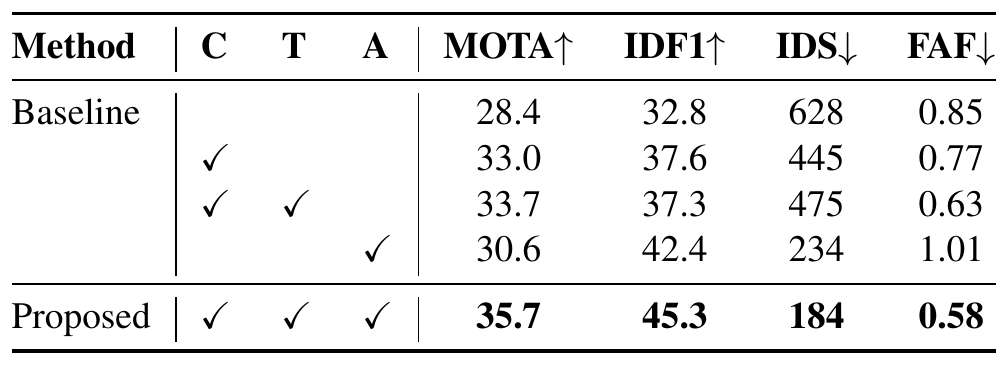
The baseline is the plainest setup, Kalman filter prediction plus IoU matching, in other words SORT's recipe.
- Using the classifier to pick candidates from detection boxes and predicted boxes (C) raises MOTA from 28.4 to 33.0 and cuts ID switches from 628 to 445. Treating predicted boxes as candidates really does recover a lot of missed detections.
- Adding track confidence (T) lifts MOTA to 33.7, and false positives per frame drop from 0.77 to 0.63. Unreliable predicted boxes get suppressed, but ID switches rise slightly to 475.
- Adding only appearance features (A) lifts IDF1 sharply from 32.8 to 42.4 and cuts ID switches to 234, but MOTA is only 30.6, and false positives per frame actually rise to 1.01.
- Adding all three gives a MOTA of 35.7, an IDF1 of 45.3 and 184 ID switches, the best on all four metrics.
The first two mainly improve the detection-related metrics, and the appearance features mainly improve the identity-related ones. Only with both sides combined does everything fall into place.
The appearance features themselves were compared too. The table below, compiled from Table 2 of the paper, swaps in different appearance representations within the same framework:
| Appearance | Dims | MOTA | IDF1 | ID switches |
|---|---|---|---|---|
| None | – | 33.7 | 37.3 | 475 |
| Color histogram | 750 | 34.9 | 38.6 | 250 |
| HOG | 1152 | 34.6 | 38.5 | 317 |
| Color + HOG | 1902 | 34.7 | 39.3 | 307 |
| re-ID feature | 512 | 35.7 | 45.3 | 184 |
Hand-crafted features help as well, but their IDF1 tops out at around 39; the learned re-ID feature has the fewest dimensions, yet its IDF1 is 6 points higher.
Speed
The authors measure per-frame processing time on the most crowded sequence, MOT16-03 (over 50 people per frame on average). Cropping every candidate box and classifying each one with SqueezeNet plus two fully connected layers takes 206.2 milliseconds per frame; switching to R-FCN with shared score maps brings it down to 66.3 milliseconds.
The MOT16 test set
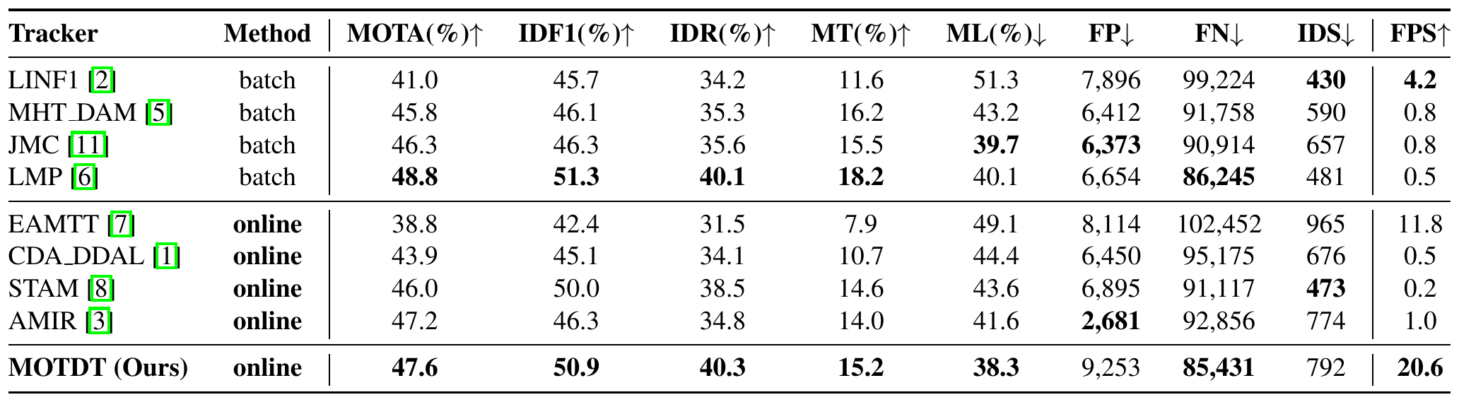
With public detections, MOTDT's MOTA of 47.6 and IDF1 of 50.9 are both the highest among the online methods in the table, and its ML of 38.3% and FN of 85,431 are even the lowest in the whole table. It runs at 20.6 FPS, which the authors put at roughly 5 to 20 times faster than most existing methods; most methods in the table manage only 0.2 to 1 frame per second, so the gap is actually larger. Compared with the best offline method, LMP, its MOTA is only 1.2 points lower, while it runs 40 times as fast.
Two columns don't look so pretty, though. FP is 9,253, more than three times AMIR's 2,681; ID switches are 792, also higher than STAM's 473 and LMP's 481. Our guess is that treating predicted boxes as candidates recovers missed detections but also keeps some boxes that shouldn't exist.
What came after
In their conclusion, the authors write that in the future they want the classifier and the appearance features to share convolutional layers, for further efficiency gains.
The following year, Zhongdao Wang and colleagues at Tsinghua University published JDE, which outputs detection boxes and re-ID features at the same time from a single detection network. Its official code also associates by matching first on appearance plus motion, then on IoU for whatever is left. The year after that, FairMOT adopted the same two-stage association. The other half of MOTDT, "treat predicted boxes as candidates too," wasn't carried over into FairMOT.
In 2021, ByteTrack included MOTDT in its comparisons, running it with the same YOLOX detector on the MOT17 validation set. MOTDT's MOTA is 75.8 and BYTE's 76.6. ByteTrack's authors argue that using predicted boxes as track boxes, as MOTDT does, may make positions drift little by little; BYTE instead fishes people back out of low-score detection boxes, which gives more accurate positions. The two papers tackle the same problem (how to keep from losing people when the detector is unreliable), but reach for different material to patch the holes.
Conclusion
MOTDT treats both detection boxes and track-predicted boxes as candidates, gives them a unified score with a position-sensitive fully convolutional classifier, and uses track confidence to push down predictions that haven't been confirmed for too long. During association, appearance is used only on detection boxes, and the rest is left to IoU. This approach reached the highest MOTA and IDF1 among online methods on MOT16 at the time, at 20 frames per second.
If you want to add re-ID to your own tracker, hierarchical association is a very practical starting point. Appearance features come only from trustworthy detection boxes, and predicted boxes are only there to fill in. The rule is simple, yet it directly avoids the mistake of "remembering someone else's face as your own."
As for "candidate selection," which takes up half the title, later trackers have hardly ever brought it up again.