Original paper
What is being transferred in transfer learning?
- Publication
- NeurIPS 2020Conference
- First submitted to arXiv
- arXiv:2008.11687
Cite this paper · BibTeX
The citation identifies the linked source version. It cites the original paper and its authors.
@misc{modeltuningwhatistransferred2020,
  title = {{What is being transferred in transfer learning?}},
  author = {Behnam Neyshabur and Hanie Sedghi and Chiyuan Zhang},
  year = {2020},
  eprint = {2008.11687},
  archivePrefix = {arXiv},
  url = {https://arxiv.org/abs/2008.11687}
}
Fine-tuning from ImageNet-pretrained weights is practically the standard opening move in computer vision.
People use it for photo classification, for medical images, even for hand-drawn doodles. Everyone knows it works, and the usual explanation is “feature reuse,” meaning that pretraining learns edges, textures and shapes and downstream tasks use them as they are.
But this explanation has an obvious hole. Chest X-rays look nothing like ImageNet photos, and doodles are just a few strokes. Why does pretraining still help?
Neyshabur, Sedghi and Zhang at Google designed a set of experiments that break “what exactly does pretraining carry over” into several measurable questions. One of the answers later became an important basis for model merging.
Defining the problem
The authors divide models into four kinds, and these abbreviations come up throughout:
- P: the ImageNet-pretrained model.
- RI: a randomly initialized model.
- P-T: a model that starts from P and is fine-tuned on the target data.
- RI-T: a model that starts from RI and is trained directly on the target data.
The target tasks are four datasets at different distances from ImageNet: DomainNet's real (real photos), clipart and quickdraw (doodles drawn by players of Google's “Quick, Draw!” game), plus CheXpert chest X-rays. The further down the list, the less they resemble natural photos.
DomainNet has 345 object categories in each domain, and the authors sample 50,000 images from each domain for training and 50,000 for testing. For CheXpert, they draw two sets of 50,000 from the training set to serve as training and test sets; the task is to identify five chest conditions.
Every model is a ResNet-50 with Fixup initialization and all BatchNorm layers removed.
There are three questions to answer. How much of the benefit of pretraining comes from feature reuse? How do P-T and RI-T differ in parameter space? Which parts of the network are actually being transferred?
Solving the problem
Learning curves first
On all four target tasks, P-T beats RI-T and converges much faster. The gap is largest on real, which fits the feature-reuse intuition, since real photos are the closest to ImageNet.
But CheXpert and quickdraw improve as well. At least on these two tasks, “reusing visual features” does not seem to explain everything.
Shuffling the images
To isolate feature reuse, the authors run a very direct experiment. They cut the target images into blocks of equal size and shuffle the positions of the blocks at random.
Blocks of 224×224 amount to no shuffling at all; the smaller the blocks, the more thoroughly object shapes and structure are destroyed. At 1×1 every pixel is shuffled, but the three RGB values of each pixel still move together, so the authors add a “*” setting in which the pixels of each channel move independently, even into other channels.
At “*”, the image is nothing but a distribution of pixel values with all visual structure gone. The edges and textures learned in pretraining cannot possibly be of any use.
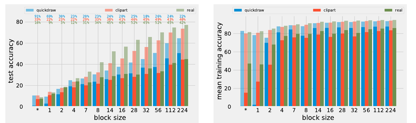
The three rows of small numbers above the left panel are the part most worth reading. They are the relative accuracy gap , which is the share of the accuracy that pretraining contributes.
For real (green), the gap is 42% without shuffling and falls to 3% once the blocks shrink to 2. For clipart (red), it also drops from around 40% to just over 20%. The smaller the blocks, the smaller the benefit of pretraining, and that is evidence of feature reuse.
The quickdraw curve (blue) behaves differently. It stays at roughly 20% to 25% for most block sizes and does not fall as the blocks shrink; at 1×1 and “*”, the number actually jumps to 69% and 91%. RI-T barely learns anything in those two settings, which is why the relative gap gets so large.
The right panel is about training speed. P-T's training accuracy holds steady however small the blocks get, while RI-T's drops sharply with small blocks. In the “*” setting, quickdraw's RI-T has an average training accuracy close to zero, while P-T is still above 80%.
This figure splits the benefit of pretraining into two parts:
- Feature reuse: the more the target resembles the pretraining data, the larger its contribution, and it disappears once image structure is destroyed.
- Low-level statistics: even when only the distribution of pixel values remains, pretrained weights still make training much faster, and sometimes improve final accuracy too.
The authors use the term “low-level statistics” for the latter to stress that it carries no visual or semantic structure. The paper does not go on to isolate which property of the pretrained weights helps optimization, such as the scale of the weights.
Opening up the models
Next, the authors compare the trained models themselves.
Overlapping mistakes. Two P-T models (fine-tuned with different random seeds) make very similar mistakes, whereas P-T and RI-T disagree on many more. Looking through DomainNet examples, the authors find that the samples P-T gets wrong and RI-T gets right are mostly ambiguous images, while the samples P-T gets right and RI-T gets wrong include quite a few easy ones.
Feature similarity. The authors use CKA (centered kernel alignment) to compare the features two models output at the same layer. Here is Table 1, on CheXpert:
| Comparison | conv1 | layer 1 | layer 2 | layer 3 | layer 4 |
|---|---|---|---|---|---|
| P-T & P | 0.6225 | 0.4592 | 0.2896 | 0.1877 | 0.0453 |
| P-T & P-T | 0.6710 | 0.8230 | 0.6052 | 0.4089 | 0.1628 |
| P-T & RI-T | 0.0036 | 0.0011 | 0.0022 | 0.0003 | 0.0808 |
| RI-T & RI-T | 0.0016 | 0.0088 | 0.0004 | 0.0004 | 0.0424 |
Two P-T models are similar at every layer. Two RI-T models also reach decent accuracy, yet their features are barely similar at all. Moving toward the output, the similarity between P-T and P falls, which shows that fine-tuning mainly changes the higher layers.
Parameter distance. Two P-T models are also close in parameter space. On CheXpert, the distance between two P-T models is about 200, and between two RI-T models about 255. Across DomainNet's three domains the contrast is starker, with two P-T models 178 to 219 apart and two RI-T models 777 to 822 apart.
The same basin
This is the section most relevant to model merging. The authors linearly interpolate between two solutions, and , and look at how the models along the path perform:
If the two solutions sit in the same flat basin, the interpolation path stays inside the basin too, and performance does not drop.
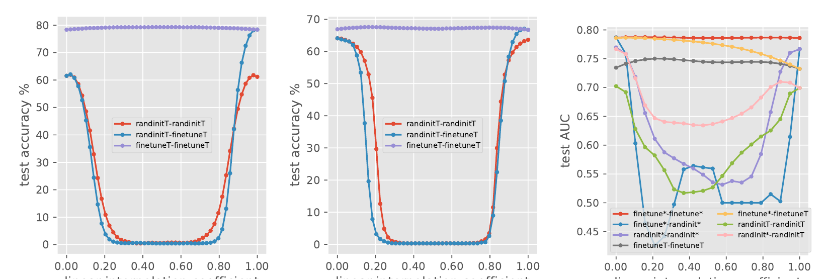
The two plots on the left are easy to read. On real, the purple line between two P-T models stays near 80% from start to finish, while the red line between two RI-T models drops close to zero in the middle. The quickdraw plot shows the same pattern.
More interesting still, the authors give two RI-T models exactly the same random initial values, so that only the randomness of training differs, and a barrier still appears. A shared starting point is not enough on its own; that starting point has to be pretrained. On CheXpert, RI-T even shows a small barrier between the best checkpoint and the final checkpoint of the same training trajectory, while P-T does not.
The authors also try to give “basin” a formal definition, which they call an -basin. For a convex set to count as a basin, most points inside it must have a loss close to the average, and adding Gaussian noise at the set's boundary or extending outward from it must raise the loss noticeably. With test error as the loss, the basin containing two P-T models has parameters on real, on clipart and on quickdraw. For two RI-T models, no reasonable places them in the same basin.
Models in the middle of the interpolation path are sometimes even slightly better than both ends. For later research, this is the paper's most useful observation. Fine-tuned models that start from the same pretrained point can be averaged directly.
Which layers transfer
Following Zhang et al., the authors rewind one module of a trained network to its initial values, keep the other modules at their trained values, and see how much performance drops. Modules whose rewinding causes a large drop are called “critical” modules.
On CheXpert, the distribution of critical modules for P-T is similar to that of standard supervised training. The only difference is that the fully connected layer becomes critical for P-T, which makes sense, because the classification head is trained only for the new task.
The authors then extend Chatterji et al.'s definition of module criticality, measuring how much noise a module's parameters can tolerate along the path from their initial values to their optimal values. The closer a module is to the output, the narrower its valley and the less it can be disturbed; modules near the input are more forgiving. This echoes the old observation that “lower layers learn general features and higher layers learn task-specific features,” and it also indicates that feature reuse happens mainly in the layers near the input.
RI-T's modules also show a turning point along the path, where the valley alternately widens and narrows. The authors guess that this may be related to switching basins partway through training, but cannot really explain it.
How long to pretrain
The last experiment is very practical. The authors fine-tune from the checkpoint saved at every epoch of ImageNet pretraining; pretraining decays its learning rate at epochs 30 and 60.
The overall trend is that later checkpoints are better, but a few details stand out:
- Checkpoints just before and after a learning-rate decay (for example 29, 30 and 31) give similar fine-tuning results. Pretraining accuracy jumps substantially at the decay, but the downstream benefit does not jump along with it.
- The training-speed benefit saturates at around checkpoint 10, while final accuracy on real and clipart keeps improving until around checkpoint 60. For quickdraw, final accuracy stops improving early, at checkpoint 10.
- A pretrained model's own accuracy is therefore not necessarily a reliable indicator of how well it transfers.
The authors connect these results to the basin observation. Early pretraining checkpoints are still outside the final basin. Once training enters the basin, it makes little difference which checkpoint fine-tuning starts from, so fine-tuning can begin from a relatively early checkpoint.
Discussion
This is an analysis paper that proposes no new method. Its value lies in a handful of observations you can put to use.
Keep the scope of the evidence in mind. Every experiment uses a single architecture (ResNet-50 without BatchNorm) and a single pretraining source (ImageNet), with four image datasets as target tasks. In the related-work section, the authors state plainly that transfer learning in NLP differs in the nature of the data, the pretraining method and the distribution gap, and that this paper studies only vision.
“Low-level statistics” is also only a description. It tells us that some benefit remains after the images are shuffled, but the paper does not test separately whether pixel distributions, weight scale or some other optimization property is responsible. For the turning point in module criticality, too, the authors leave only a guess.
The “same basin” observation had the largest impact. In their conclusion, the authors mention it in a single sentence, noting that averaging models within the same basin does not hurt performance. Two years later, Model Soups turned it into a practical method, directly averaging many models fine-tuned with different hyperparameters, and cited this paper as the basis for why averaging works.
Conclusion
Pretraining carries over two kinds of things. One is visual features, which help more the more the downstream data resembles ImageNet. The other is low-level statistics that survive even when the pixels are scrambled, and these mainly make training faster.
Fine-tuned models that start from the same pretrained weights have similar features, sit close together in parameter space, and show no barrier under linear interpolation. Models trained from scratch cannot manage this even when they share the same random initial values.
Next time you have two sets of weights fine-tuned from the same pretrained model, don't rush to pick one. Try averaging them; you may find that neither beats the one in the middle.