Original paper
The Role of Permutation Invariance in Linear Mode Connectivity of Neural Networks
- Publication
- ICLR 2022Conference
- First submitted to arXiv
- arXiv:2110.06296
Cite this paper · BibTeX
The citation identifies the linked source version. It cites the original paper and its authors.
@misc{modelmergingpermutationinvariance2021,
  title = {{The Role of Permutation Invariance in Linear Mode Connectivity of Neural Networks}},
  author = {Rahim Entezari and Hanie Sedghi and Olga Saukh and Behnam Neyshabur},
  year = {2021},
  eprint = {2110.06296},
  archivePrefix = {arXiv},
  url = {https://arxiv.org/abs/2110.06296}
}
Around 2018, research on loss landscapes told us something strange.
Between two networks trained from different random initializations, you can find a curved path along which the loss stays low; connect them with a straight line, though, and the loss still shoots up in the middle. The detour works, but the straight line is blocked.
Entezari, Sedghi, Saukh and Neyshabur at TU Graz and Google came up with a possible reason. The hidden units of a neural network have no fixed order. Rearrange the neurons within a layer and the network computes exactly the same function, yet its parameter vector becomes a different point. Perhaps two networks hit a wall on the straight line simply because their neurons are “sitting in the wrong seats.”
They wrote this idea up as a conjecture and openly admitted that it was a bold one.
Defining the problem
Measuring the barrier
Let be the network's loss at a given set of parameters (training error, for example). The linear interpolation barrier between two parameter sets and is defined as
The first term is the loss of the interpolated model, and the second is the linear interpolation of the two endpoint losses. Their difference measures “the extra amount above what the straight line would predict.”
This differs slightly from Frankle et al.'s definition. Frankle uses the average of the two endpoint losses, , as the baseline. When the endpoint losses are equal, the two definitions agree; when they differ, this version does not count “loss changing linearly from one end to the other” as part of the barrier.
When , the two networks are said to have linear mode connectivity (LMC). The authors found experimentally that measuring once at differs from taking the supremum over the whole path by less than , so the later figures report only the midpoint value.
What the barrier depends on
Before proposing the conjecture, the authors ran a survey. The architectures are a single-layer MLP, a Shallow CNN with two convolutional layers, VGG and ResNet; the datasets are MNIST, SVHN, CIFAR-10 and CIFAR-100. For each setting they train 10 models with different seeds and measure the training-error barrier on 5 random pairs.
- Width: the barrier first rises with width, then starts to fall past a certain width, a shape much like double descent. Comparing against test error, the authors find that the barrier peaks at roughly the width where the model can just fit the training data. Simpler datasets (MNIST, SVHN) start to fall earlier than CIFAR.
- Depth: with MLP and Shallow CNN layers fixed at width , every added layer makes the barrier noticeably higher. The barriers of VGG and ResNet stay stuck at a high level and do not change with width.
- Task difficulty: the MLP's barrier is only 0.0174 on MNIST but 0.7965 on CIFAR-100; the Shallow CNN goes from 0.0161 to 0.4861. For shallow networks, the barrier is strongly positively correlated with test error. ResNet18 and VGG16 sit between 0.84 and 0.99 on all four datasets, with low test error and yet very high barriers.
The survey's conclusion is that width lowers the barrier and depth raises it. These phenomena call for an explanation.
Solving the problem
Two invariances
If a network still represents the same function after some transformation, the network is said to be invariant to that transformation. Two kinds are common.
The first is the positive homogeneity of ReLU. Multiply a neuron's incoming weights by and divide its outgoing weights by , and the function stays the same. The authors consider this invariance unimportant, because SGD's implicit bias tends to balance the magnitudes of the weights across layers, so training converges to a particular scaling.
The second is permutation invariance. Rearranging the hidden units of layer turns the parameters into
where is a permutation matrix, and the input and output layers are not permuted. reorders this layer's outputs, and undoes the previous layer's permutation. For SGD, every permutation is equally likely, so the effect of permutations on the loss landscape deserves serious attention.
Let's check this with a single-hidden-layer network. The hidden layer has units. Reorder the rows of the first-layer weights, the biases and the columns of the second-layer weights with the same permutation:
def permute(params, p):
    W1, b1, W2, b2 = params        # W1: [h, d], b1: [h], W2: [10, h], b2: [10]
    return [W1[p], b1[p], W2[:, p], b2]
In the small experiment later in this note, networks of width 16, 64 and 256 are each randomly permuted once, and torch.allclose compares their outputs on the whole dataset before and after the permutation. All three comparisons return True. The function is exactly the same, but in parameter space these are two points far apart.
A single layer of width already has possible orderings. The same function has an astronomical number of equivalent copies in parameter space.
The conjecture
In plain terms, the authors' conjecture reads as follows:
Most SGD solutions belong to a set ; once suitable permutations are applied to the elements of , linear interpolation between any two of them has no barrier.
The formal version adds a width condition. There exists a width such that, for any sufficiently wide network, there is a set of solutions and a function that assigns permutations, so that any two solutions in have approximately zero barrier after permutation, and SGD solutions fall in with high probability.
If the conjecture holds, the many seemingly separate basins in the loss landscape are really just copies of a single basin, replicated by permutation.
Theory: only the simplest case is proven
The authors prove a very restricted version. Take a single-hidden-layer, fully connected ReLU network at random initialization, with weights drawn from a specified uniform distribution. With high probability there exists a permutation such that the error between the output of the interpolated network and the interpolation of the two endpoint outputs is only
is the number of hidden units and is the input dimension. When the network is wide enough, the error goes to zero.
The theorem covers only initialization, not trained networks. The in the exponent also shows that the required width grows extremely fast as the input dimension increases. The authors themselves say that a more involved proof might extend to the NTK regime, but they leave that for future work.
Experiments: too many permutations to search, so test it another way
Direct verification requires searching over permutations, but their number grows factorially with width. The authors tried brute-force search and could only go as far as a single-hidden-layer MLP with 16 neurons, which is already permutations.
Even with a smarter search algorithm, a failure cannot tell us whether the algorithm is too weak or whether no such permutation exists at all.
So the authors approach it from another angle. Given an SGD solution , collect all of its permutations into a set
always satisfies the conjecture, because every element is a permuted copy of ; undo the permutation and the barrier is zero. The paper calls “our model” and the actual set of SGD solutions “the real world.”
What remains is to check whether and behave the same way. Suppose the barrier between an independently trained solution and is about the same as the barrier between and “a random permutation of ,” across widths, depths and datasets. Then “ is really some permutation of plus a small perturbation” is a reasonable explanation.
Try it yourself
This argument can be reproduced at a very small scale.
The figure below comes from a small experiment run separately for this note; it is not a result from the paper. The data is sklearn's built-in 8×8 handwritten digits (1,797 images), and the model is a single-hidden-layer ReLU MLP. Two models, A and B, are trained with different seeds, both reaching a training loss of around 0.001. We then compare three linear interpolations: A to B, A to “a randomly permuted A,” and A to “an aligned B.”
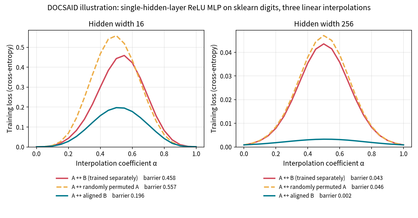
Look at the red and orange lines first. A and B are separately trained models, while A and the permuted A are the same function, yet the two curves peak at about the same height. This is the paper's core observation. The barrier that independent training creates is about as high as the barrier created by “just swapping seats.”
The teal line is our own addition. B's hidden units are matched one-to-one to A's by activation correlation using the Hungarian algorithm, and then the two are interpolated. At width 16 the barrier falls from 0.458 to 0.196; at width 256, from 0.043 to 0.002. This alignment method comes from later research and is not the search method this paper uses. It is here to show you how much “putting units in the right seats” can actually achieve.
At width 64, the three barriers are 0.094, 0.070 and 0.006. The wider the network, the lower the barriers, and the closer to zero they get after alignment, consistent with the trend in the paper's survey.
The paper's evidence
Back to the paper. The authors compare and on MLPs and Shallow CNNs, and across widths, depths and datasets the two barrier curves almost overlap.
Next comes search. The authors use simulated annealing to find permutations, an approximation algorithm commonly used for the traveling salesman problem. There are two versions:
- SA1: directly minimize the average pairwise barrier among five solutions.
- SA2: first average the permuted solutions into a single model, then minimize the training error of that averaged model.
The two perform about the same and SA2 is much cheaper, so only SA2 is used from then on. But in the setting where five solutions are aligned at once, it barely lowers the barrier.
The authors therefore shrink the search space to just two solutions, fixing and permuting only . With that, the barriers of MLPs and Shallow CNNs on MNIST and SVHN drop clearly, and the single-layer MLP on MNIST even reaches zero at every width. More importantly, the barriers of and remain almost the same both before and after search. Where search succeeds on , it also succeeds on ; where it fails on , it fails on as well.
Across all the experiments, the authors trained more than three thousand networks. The authors plot them in a density map, and the barriers of “the real world” and “our model” fall roughly along the diagonal.
Discussion
The way this paper argues is interesting. It does not prove the conjecture. Instead, it designs a set of experiments in which “if the conjecture were wrong, we should see a difference,” and no difference shows up. The authors word it carefully too, saying that these attempts “failed to falsify” the conjecture.
The strength of the evidence, however, has to be judged piece by piece.
The most convincing part concerns shallow networks. On MLPs and Shallow CNNs, and look alike both before and after search, and search really can bring the barrier down to zero on simple datasets.
The evidence for deep networks is weaker. VGG and ResNet have high barriers on both and , and simulated annealing finds no barrier-reducing permutation on either side. “Failure on both sides” is compatible with the conjecture, but it also cannot tell whether the search algorithm is too weak or whether deep networks have some other barrier altogether. The authors also admit that the size of the search space is the paper's biggest limitation, and that every experiment is in image recognition.
The argument itself carries an implicit premise as well. and being similar in “barrier under direct interpolation” and “barrier after search” does not guarantee that they are also similar in “barrier under the optimal permutation,” and the latter is what the conjecture is really about.
Later research filled in the deep-network piece. Git Re-Basin switched to weight matching and, on ResNets widened many times over, achieved zero barrier between two independently trained CIFAR-10 models for the first time. It also constructed a counterexample from non-SGD solutions, showing that the qualifier “SGD solutions” in the conjecture cannot be dropped. REPAIR, the next paper we look at, found another reason deep networks keep a barrier after alignment, and traced the problem to the variance of the activations after interpolation.
Conclusion
The paper puts forward a simple idea. Many seemingly different basins in the loss landscape may be nothing more than permuted copies of a single basin.
Its theory covers only the single-hidden-layer case at random initialization. Its experiments rely on a clever substitute, “simulating independently trained solutions with permutations of one solution,” and give fairly consistent support on shallow networks.
You don't need a big model to get a hands-on feel for this. Train two small MLPs, shuffle the hidden units of one of them however you like, and interpolate it against its original self. You'll see a mountain about as high as the one between two independent models.