Original paper
From Intuition to Investigation: A Tool-Augmented Reasoning MLLM Framework for Generalizable Face Anti-Spoofing
- Publication
- CVPR 2026Conference
- First submitted to arXiv
- arXiv:2603.01038
Cite this paper · BibTeX
The citation identifies the linked source version. It cites the original paper and its authors.
@misc{faceantispoofingtarfas2026,
  title = {{From Intuition to Investigation: A Tool-Augmented Reasoning MLLM Framework for Generalizable Face Anti-Spoofing}},
  author = {Haoyuan Zhang and Keyao Wang and Guosheng Zhang and Haixiao Yue and Zhiwen Tan and Siran Peng and Tianshuo Zhang and Xiao Tan and Kunbin Chen and Wei He and Jingdong Wang and Ajian Liu and Xiangyu Zhu and Zhen Lei},
  year = {2026},
  eprint = {2603.01038},
  archivePrefix = {arXiv},
  url = {https://arxiv.org/abs/2603.01038}
}
When Idiap released the Replay-Attack dataset in 2012, the baseline method was LBP. Each pixel compares its brightness with its eight neighbors. A neighbor that is no darker than the center scores 1 and a darker one scores 0, together forming an 8-bit code, and the codes across the whole face are then counted into a histogram. Paper fibers and screen pixel grids have textures unlike skin, so the histogram comes out different too.
More than a decade later, face anti-spoofing has moved on to multimodal large language models. I-FAS has the model answer "Is this photo of a real person?", first saying Yes or No, then adding a one-sentence explanation. The trouble is that the explanation often looks like this:
This is a picture of a man wearing glasses.
All true, but it has little to do with whether the face is real.
Zhen Lei's team at the Institute of Automation, Chinese Academy of Sciences, joined by the Baidu group behind I-FAS, has now brought LBP back. It does not go back into the network as a feature. Instead it becomes a tool, and the large language model decides for itself when to call it up and take a look.
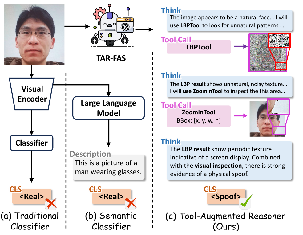
The middle column is I-FAS's output format. On the right is this paper's approach. The model takes a first look and thinks it is a live face, then calls the LBP tool, sees a patch of unnatural texture in the output image, zooms in on that patch, and finally changes its verdict to attack.
Defining the Problem
I-FAS recast anti-spoofing as visual question answering, and its cross-dataset results beat the CLIP-family methods by a wide margin. The authors believe its ceiling lies in that one-sentence description. Citing earlier research, they point out that multimodal large language models already have some blind spots for low-level visual features, and since the training objective asks only for a short explanation, what the model learns is mostly visible semantic cues such as "wearing a mask" or "holding a screen." The moiré left by recapturing a screen, a printer's halftone dots, and the faint reflections of mask materials are hard to fit into one sentence, so they never get learned.
A table in FaceCoT's appendix makes this even clearer. Judging Rose-Youtu's attack images zero-shot, a general-purpose model recognizes most of the masks, yet does not catch a single print or screen replay.
So how do you get a large language model to look at those pixel-level traces?
Traditional anti-spoofing has always dealt with this, and LBP, HOG, and FFT were the usual tools back then. On the other side, recent multimodal models can already call external tools partway through their reasoning; DeepEyes, for example, lets the model decide for itself which part of the image to zoom into. The authors connect the two, letting the model call these classic image operators while it reasons.
Solving the Problem
The Toolbox
The authors prepare six tools in four categories:
- ZoomIn: given a box, crops that region and enlarges it.
- Texture: LBP, which checks whether the skin texture looks natural; paper and mask materials often give themselves away here.
- Frequency: FFT and the wavelet transform, which check the frequency distribution for anomalies; screens and printed material often carry periodic signals.
- Structure: HOG and Laplacian edge detection, which look at boundaries and gradients; mask edges and screen bezels surface here.
Every tool outputs an image, which is fed back to the model. So when the model "looks at a tool result," it is actually looking at an LBP code map, a spectrum, or an edge map.
Why can an FFT image reveal a screen? The illustration below converts two 64×64 images into spectra. The top row is a smooth brightness bump standing in for a face photographed directly; the bottom row overlays the same face with vertical stripes that repeat every 8 pixels, simulating the periodic pattern that shows up when you photograph a face off a screen.
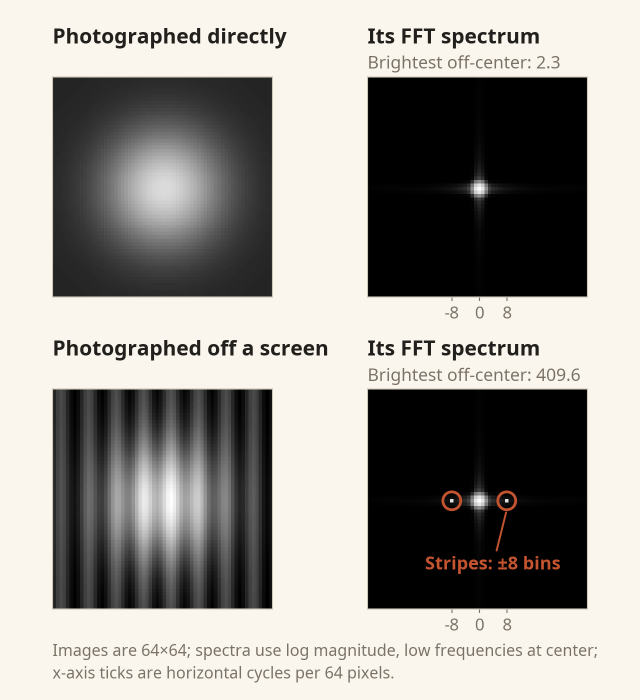
The top-right spectrum has only the central blob, the low-frequency energy of the smooth brightness bump, which grows darker with distance from the center. The bottom right has two extra small bright spots that land exactly at −8 and +8 on the horizontal axis. An image 64 pixels wide with one period every 8 pixels holds exactly 8 periods, so the spots sit 8 bins from the center, one on each side, and their magnitude is more than a hundred times that of the brightest off-center point in the direct shot.
In the bottom-left image, the stripes blend into the face's brightness and are hard to separate; in the spectrum, they concentrate into two points you can spot at a glance. Real moiré has messier directions and periods, so its spectral spots spread out, but the principle is the same. TAR-FAS's FFT tool returns exactly this kind of spectrum, and what the model has to learn is to look for bright spots away from the center.
The paper does not give the implementation parameters of the tools; this figure only shows what the FFT tool's output looks like.
ToolFAS-16K: Demonstrations from a Teacher Who Knows the Answer
At first the model does not know how to use tools, so it needs demonstrations. The authors picked 16,172 images from CelebA-Spoof, nearly half of them live and the rest covering 10 attack types, and had Gemini-2.5 Pro write out tool-using reasoning turn by turn.
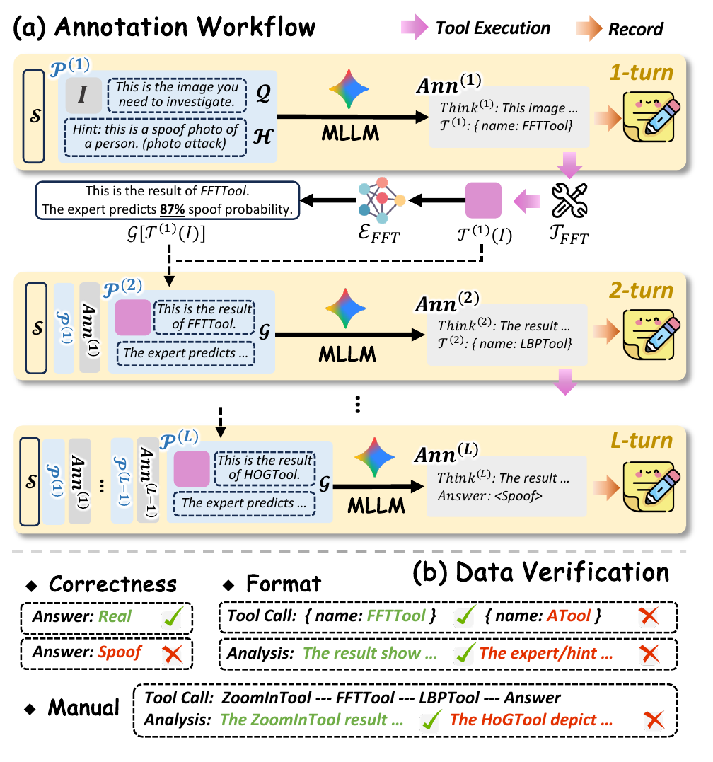
Start with turn 1 in the figure. Besides the image and the sentence "This is the image you need to investigate," Gemini receives a hint that states outright whether the image is live or which kind of attack it is. The system prompt also makes clear that the final classification must agree with the hint, and that the reasoning must not mention the hint.
When Gemini asks to call a tool, the tool result goes back to Gemini, but first it is also passed to an "expert model." Each tool (except ZoomIn) has its own expert, a small CNN with only three convolutional layers. Its only input is the tool's output image; it never sees the original image, and it outputs the probability that the image contains spoof traces. The authors trained these on 4,000 CelebA-Spoof identities and tested them on 1,000, and at a threshold of 0.5 the small models reach roughly 80 to 90% accuracy. The next turn's prompt then gains a line such as "This is the result of FFTTool. The expert predicts 87% there's spoof trace."
An annotation runs for at most 6 turns and ends when Gemini gives an answer. Then come three checks. The answer must match the label; tool calls must follow the format, and the analysis must not mention the hint or the expert's probability; finally, a person confirms that the tool analysis and the conclusion connect logically. Anything that fails is annotated once more, and if it fails again, it is discarded.
So this dataset is a set of worked demonstrations for a student, written by a teacher who knows the answer in advance and has an assistant at their side calling out probabilities. The hint and the expert probabilities are filtered out by the checks, so the student never sees them. What the student learns here is how to call tools and how to write reasoning; its own ability to judge from the tool results has to be trained by reinforcement learning in the next stage.
Three Training Stages
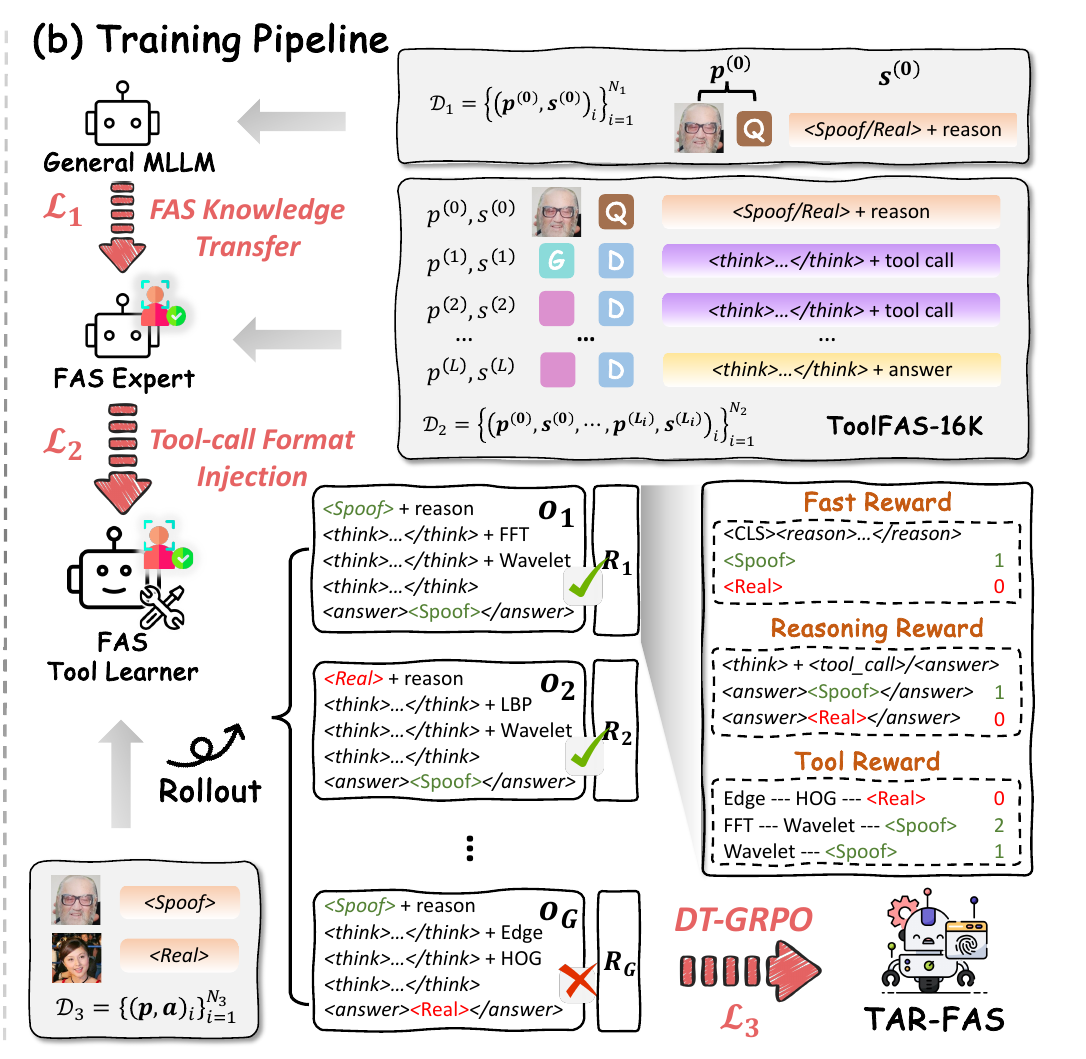
The backbone is InternVL3-8B. The figure shows three stages from top to bottom:
-
FAS knowledge transfer (KT): supervised fine-tuning on I-FAS-format data. The question is always "Is this photo of a real person?", and the answer is
<Real>or<Spoof>plus a one-sentence reason. This step first gets the general model to understand what anti-spoofing is asking. -
Tool-call format injection (FI): fine-tuning on ToolFAS-16K. The first turn of every sample is identical to the previous stage, a fast answer; only after that come the turns of thinking and tool calls. The loss function is
The first turn carries 90% of the weight. Multi-turn data is long, and if every token weighed the same, the short fast-answer segment would easily be diluted; the model would learn to use tools but forget how to classify directly.
-
DT-GRPO: reinforcement learning using only CelebA-Spoof images and their live/spoof labels, with no reasoning demonstrations needed anymore.
The first two stages use LoRA (rank 16) for up to 4,000 steps; the third stage unfreezes all parameters, with a learning rate of 1e-6, 8 sampled responses per question, up to 300 steps, and the KL penalty set to 0.
The DT-GRPO Reward
GRPO samples a group of responses to the same question, gives each response a score , then subtracts the group mean and divides by the group standard deviation to get the advantage . Responses better than average are reinforced, and those worse than average are pushed down.
In this paper, the score is a weighted sum of three terms:
- : the first-turn fast answer. A format error scores −1; otherwise a correct answer scores 1 and a wrong one 0.
- : the final answer. A reasoning format error or an invalid tool call scores −1; otherwise a correct answer scores 1 and a wrong one 0.
- : each distinct tool used adds 0.2, and calling the same tool twice counts only once; if the final answer is wrong, the whole term drops to zero.
Let's work it through for one attack image and five responses:
import numpy as np

beta_fast, beta_rsn, beta_tool, gamma = 0.1, 0.5, 0.4, 0.2

def reward(fast_ok, tools, final_ok, fmt_ok=True):
    r_fast = 1.0 if fast_ok else 0.0
    if not fmt_ok:                       # bad reasoning format or invalid tool call
        return beta_fast * r_fast + beta_rsn * -1.0
    r_rsn = 1.0 if final_ok else 0.0
    r_tool = gamma * len(set(tools)) if final_ok else 0.0   # each tool type counts once; zero if wrong
    return beta_fast * r_fast + beta_rsn * r_rsn + beta_tool * r_tool

# five responses sampled for the same attack image (label Spoof)
rollouts = [
    ("fast answer Real, checks FFT and Wavelet, switches to Spoof", reward(False, ["FFT", "Wavelet"], True)),
    ("fast answer Spoof, settles it without tools", reward(True, [], True)),
    ("fast answer Real, checks Edge and HOG, still Real", reward(False, ["Edge", "HOG"], False)),
    ("fast answer Spoof, FFT twice plus LBP", reward(True, ["FFT", "FFT", "LBP"], True)),
    ("fast answer Spoof, malformed tool call", reward(True, [], False, fmt_ok=False)),
]
r = np.array([ri for _, ri in rollouts])
adv = (r - r.mean()) / r.std()           # GRPO: normalize within the group
for (name, ri), ai in zip(rollouts, adv):
    print(f"R={ri:+.2f}  A={ai:+.2f}  {name}")
R=+0.66  A=+0.75  fast answer Real, checks FFT and Wavelet, switches to Spoof
R=+0.60  A=+0.61  fast answer Spoof, settles it without tools
R=+0.00  A=-0.72  fast answer Real, checks Edge and HOG, still Real
R=+0.76  A=+0.97  fast answer Spoof, FFT twice plus LBP
R=-0.40  A=-1.61  fast answer Spoof, malformed tool call
Putting the five responses side by side:
- Getting it right is what counts most. A correct final answer is worth 0.5, while the tool reward tops out at (at most three tool calls, all three different). A response that answers correctly without checking any tool still gets a positive advantage.
- Tools are bonus points. Among correct answers, each extra kind of tool consulted adds 0.08. The first response got the fast answer wrong and turned it around with tools, yet it still scores higher than the one that answered correctly outright.
- Calling FFT twice earns nothing extra, so the model is pushed toward "try a different tool," which is what Diverse-Tool in the name means.
- The malformed response scores negative and has the lowest advantage.
- Nothing in the reward encourages calling fewer tools. As long as the answer is right, using all three calls on three different tools scores highest. The only cap on inference cost is the rule of at most three tool calls.
At Inference Time
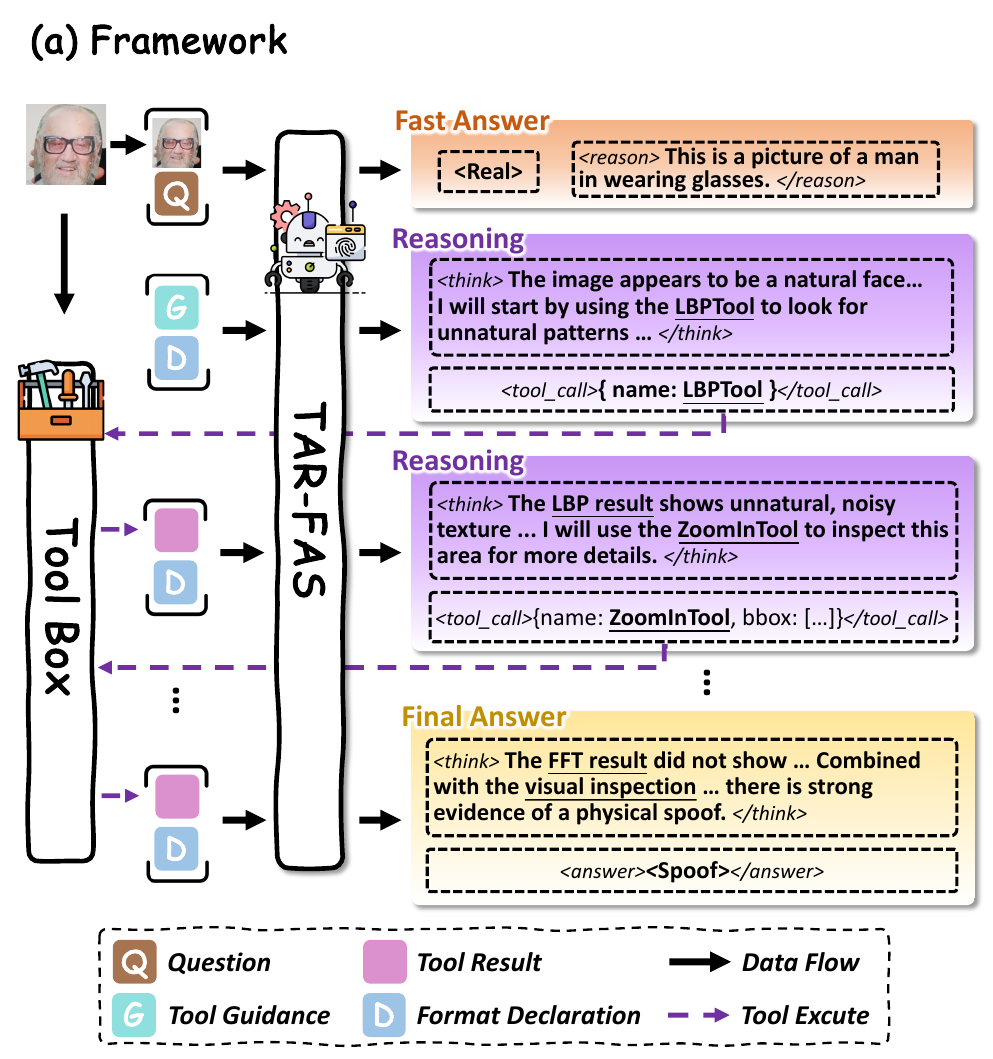
Inference has two parts. The first turn asks "Is this photo of a real person? (Do not use any tools)", and the model gives a fast answer in I-FAS format. The second turn sends in a prompt:
Wait, you should re-examine the image and give the final answer (use tools if needed).
The model starts writing <think> and emits <tool_call> when needed; an external program runs the tool and sends the result image back, and this repeats for at most three tool calls before the model writes <answer>. For HTER and AUC, the score comes from the logits of the classification token in the final answer.
There is no expert model and no attack-type hint at inference time; the model has to read the tool output images on its own.
Discussion
One-to-Eleven
The main experiment follows I-FAS's Protocol 2, training only on CelebA-Spoof and testing directly on 11 datasets, with each setting averaged over three random seeds. The inputs are aligned, cropped 224×224 faces, which InternVL upscales to 448×448 for processing.
On average, TAR-FAS has an HTER of 7.54% and an AUC of 96.67%; I-FAS has 11.30% and 93.71%, and FLIP 18.73% and 87.90%.
The per-dataset HTER (%) is as follows:
| Test dataset | I-FAS | TAR-FAS |
|---|---|---|
| CASIA-MFSD | 1.11 | 0.00 |
| CASIA-SURF-3DMask | 6.18 | 2.09 |
| HKBU-MARs-V1+ | 18.64 | 3.48 |
| HiFiMask | 28.23 | 17.97 |
| MSU-MFSD | 5.63 | 5.71 |
| OULU-NPU | 14.86 | 14.45 |
| Replay-Attack | 9.15 | 5.75 |
| Rose-Youtu | 5.52 | 3.61 |
| SiW | 4.02 | 8.35 |
| SiW-M-V2 | 10.89 | 11.72 |
| WMCA | 20.07 | 9.78 |
| Average | 11.30 | 7.54 |
The biggest gains are on datasets with mask attacks. HKBU-MARs-V1+ falls from 18.64% to 3.48%, WMCA from 20.07% to 9.78%, and HiFiMask and CASIA-SURF-3DMask both drop considerably as well. The authors specifically point out that HKBU-MARs-V1+ and CASIA-SURF-3DMask contain attack types and materials that the source data lacks.
Interestingly, the example the paper opens with is the periodic texture of a screen, and the frequency tools are aimed at prints and screens, yet on the datasets dominated by print and screen attacks the results are mixed. Replay-Attack and Rose-Youtu improve, MSU-MFSD and OULU-NPU barely move, and SiW slips from 4.02% to 8.35%. SiW-M-V2, with the most varied attack types, also gets slightly worse.
Tools and Training Stages
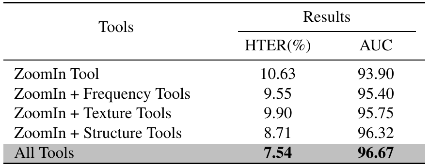
With only ZoomIn, HTER is 10.63%, already a little lower than I-FAS. Of the three tool categories, adding the structure tools alone helps most, bringing it down to 8.71%; with every tool, it is 7.54%.
This table shows that the tools are useful, but it is also a reminder that the drop in HTER from 11.30% to 7.54% does not all come from the tools. The magnifier-only version already takes part of that drop, and that part comes from the new backbone and the whole training pipeline.
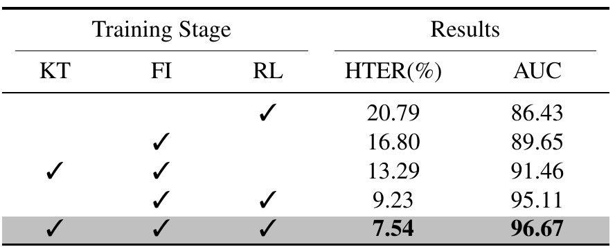
This table has more of a story to it.
- Skipping the demonstrations and going straight to reinforcement learning gives an HTER of 20.79%. In the appendix training curves, this approach's reasoning accuracy keeps oscillating in the 70% range throughout training, while the full pipeline sits around 95%. The model does not even know how to call the tools, so the reward has a hard time steering it in the right direction.
- Imitating Gemini's demonstrations alone (FI) gives an HTER of 16.80%, worse than I-FAS. Copying the teacher's worked solutions does not produce the ability to generalize.
- Adding reinforcement learning after the demonstrations brings it from 16.80% to 9.23%, the largest single step in the table.
- Adding knowledge transfer in front finally gets it to 7.54%.
A Few More Comparisons
- Fast answer vs. reasoning answer: for the same model, the first-turn fast answer has an HTER of 10.54%, and the final answer after checking with tools has 7.54%. The fast answer is already somewhat better than I-FAS, and one round of checking with tools brings it down another 3 percentage points.
- Zoom only: DeepEyes' ST-GRPO allows only ZoomIn, and its reward looks only at the format, whether the answer is right, and whether a tool was used. Switching to it gives an HTER of 9.98%, higher than DT-GRPO's 7.54%.
- The tool-call cap: in the appendix curve, raising the cap from 1 to 3 brings HTER down steadily from about 9.2% to 7.54%; loosening it to 4 pushes it back up to just over 8%. The authors attribute this to longer responses and greater sampling variance.
- Backbone and resolution: with Qwen2.5-VL-7B, feeding 224×224 directly gives an HTER of 9.45%, upscaling to 448×448 gives 8.60%, and InternVL3-8B gives 7.54%. Resolution and backbone each contribute a little, though all three numbers are below I-FAS.
The Old Protocol
The appendix also runs OCIM (the four datasets O, C, I, and M take turns as the test set). The average HTER is 1.30% against I-FAS's 1.33%, practically a tie. The four settings go both ways. OCM→I drops from 3.22% to 0.43%, but OCI→M rises from 0.32% to 2.86%.
The numbers on this protocol are already crowded around 1%, which makes it hard to separate methods any further. The training steps only have upper limits (at most 4,000 for SFT and at most 300 for RL), and the paper does not mention picking checkpoints on the target datasets; how the HTER threshold is chosen is not explained.
The Reasoning Reads Well, but It May Not Be How the Model Decided
Finally, look at the four examples the paper picked.
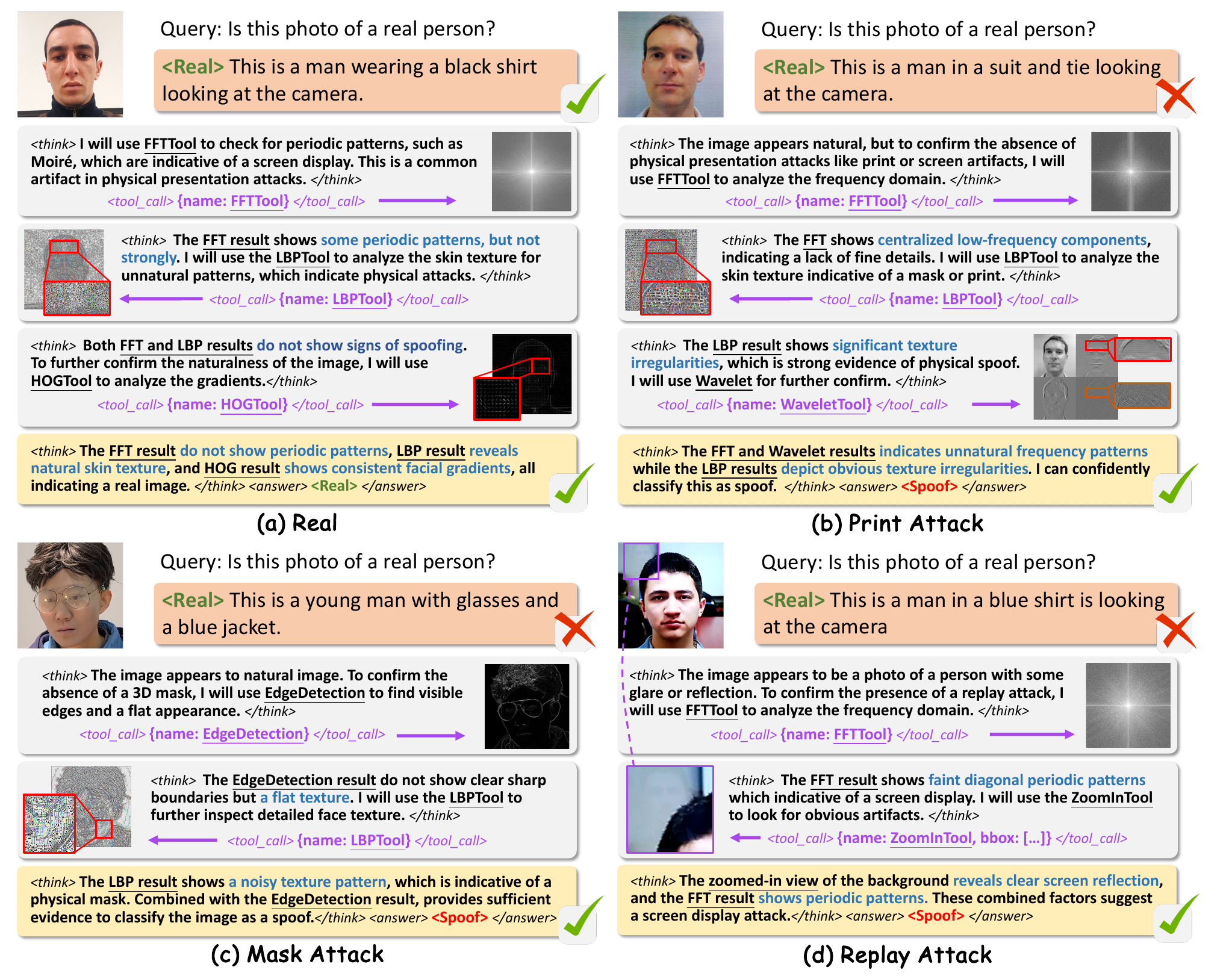
All four fast answers are Real. Three of the examples are attacks, turned around with tools. The authors observe that the model favors the frequency tools for prints and screens and the structure tools for masks, while it uses the texture tool for every kind of attack.
Read the live example in (a) more closely. After the FFT check, the model writes "The FFT result shows some periodic patterns, but not strongly"; in the final summary, this becomes "The FFT result do not show periodic patterns." The earlier hedge is gone by the conclusion, and the whole chain of reasoning has been tidied into a clean story.
It doesn't change the answer here, but it is a reminder that the written reasoning and the cues the model actually relies on are not necessarily the same thing. The paper does not test whether the tool results really sway the decision, for example by swapping the tool output for an unrelated image and seeing whether the answer changes.
There are two more things the paper does not provide, and they will certainly come up in deployment. One is inference time. An 8B model gives a fast answer, then goes back and forth for up to three more rounds, reading a new tool image each round. A typical liveness model on a phone runs a CNN once, so you can imagine the gap, but the paper does not measure it. The other is the code, which has not been released yet.
Conclusion
TAR-FAS lets a multimodal large language model call classic operators such as LBP, FFT, and HOG partway through its reasoning. Trained only on CelebA-Spoof and tested on 11 datasets, it lowers the average HTER from I-FAS's 11.30% to 7.54%, with the biggest gains on the mask datasets.
The thing most worth taking away from this paper is that one step in the ablation table. Imitating Gemini's demonstrations alone scores worse than I-FAS; the same model followed by GRPO that looks only at live/spoof labels drops from 16.80% to 9.23% HTER. The demonstrations teach how to use the tools; how well they get used is trained by reinforcement learning.
The appendix holds one more small finding. Those little expert models, with only three convolutional layers and looking only at LBP or FFT output images, already reach 80 to 90% accuracy on CelebA-Spoof. In the paper, their only job is passing notes to Gemini during annotation; they never take the field at inference.
As for whether to put an 8B model into a face-scan door, let's wait until the code is out and someone has measured the latency.