Original paper
An Unbiased Benchmark for Domain Generalization Face Anti-Spoofing
- Publication
- SIBGRAPI Workshops 2025Workshop
Cite this paper · BibTeX
The citation identifies the linked source version. It cites the original paper and its authors.
@inproceedings{faceantispoofingunbiaseddgfas2025,
  title = {{An Unbiased Benchmark for Domain Generalization Face Anti-Spoofing}},
  author = {Raul Almeida and Bruno Kamarowski and Bernardo Biesseck and Luiz Coelho and Roger Granada and David Menotti},
  year = {2025},
  booktitle = {SIBGRAPI Workshops},
  url = {https://sol.sbc.org.br/index.php/sibgrapi_estendido/article/view/38278}
}
For cross-dataset face anti-spoofing, the most common benchmark in recent years has been OCIM. There are four datasets, OULU-NPU (O), CASIA-FASD (C), Replay-Attack (I), and MSU-MFSD (M); each time, three are used for training and one for testing, as in OCI→M. From 2019 to 2025, the HTER on this benchmark fell from nearly 18% all the way to below 1%.
Raul Almeida, David Menotti, and colleagues at the Federal University of Paraná in Brazil, together with researchers from the Brazilian identity verification company unico, went back to look at how these numbers were measured. Their answer is in the title. The current benchmark is biased.
This is a short work-in-progress paper, only six pages long, and its experiments are small in scale, but it asks its question very directly.
Defining the Problem
In a standard machine learning workflow, the data is split three ways. The training set updates the weights, the validation set decides when to stop and which hyperparameters to use, and the test set is looked at once, only after everything has been finalized.
OCIM has only two. Three source datasets are used for training, and the fourth plays the role of both validation set and test set. During training, the model is evaluated on the test set after every epoch, and the best-performing epoch is reported at the end. The authors point out that this amounts to peeking at the exam throughout training.
Why does this matter? Because in deployment there is no exam at all. Once a model goes live, it meets new phones, new lighting, and new attacks, and nobody hands you labels for that data in advance so you can pick the epoch that suits it best. A score picked on the test set looks better than the score you can actually get.
How much better? Let's work through an extreme case. Suppose the model's true error rate is fixed at 10% at every epoch, with no improvement at all. The test set has 40 live videos and 80 attack videos, so every HTER measurement bounces up and down because of sampling. Repeat the same experiment 2,000 times and see what “pick the lowest of N epochs” reports on average:
import numpy as np

rng = np.random.default_rng(0)
n_live, n_spoof, true_error, trials = 40, 80, 0.10, 2000

def measured_hter(epochs):
    apcer = rng.binomial(n_spoof, true_error, (trials, epochs)) / n_spoof
    bpcer = rng.binomial(n_live, true_error, (trials, epochs)) / n_live
    return (apcer + bpcer) / 2

for epochs in (1, 10, 30, 100):
    best = measured_hter(epochs).min(axis=1)        # Pick the lowest epoch in each trial
    print(f"Epochs seen: {epochs:>3}, lowest pick averages {best.mean():.1%}")
Epochs seen:   1, lowest pick averages 9.9%
Epochs seen:  10, lowest pick averages 5.8%
Epochs seen:  30, lowest pick averages 4.6%
Epochs seen: 100, lowest pick averages 3.6%
The model has not changed at all. The more times you look at the test set, the prettier the number you pick. Look 100 times, and a 10% model can report 3.6%. In real training, the models at different epochs genuinely vary in quality, so picking the best one is not pure luck. But as long as the choice is based on the test set, that share of luck gets mixed into the reported number, and afterward there is no way to separate it out.
The authors also mention that earlier studies noticed this problem but only patched it partially. SA-FAS, for example, additionally reports the mean of the last 10 epochs, and some papers add metrics closer to deployment, such as TPR@FPR. These measures bring the numbers closer to reality, but the test set is still seen during training. The authors say that, to their knowledge, this is the first study to address this bias specifically and propose an alternative benchmark.
Solving the Problem
The method makes just one change. It adds one more dataset.
This fifth dataset can be used in two ways:
- Add it as a validation set: OCIM training and testing stay the same, but each epoch is evaluated on the new validation set, which is used to pick the best epoch; HTER is computed once on the original test set only after training ends.
- Add it as a test set: the original fourth dataset steps back to serve as the validation set, and the final score is measured on the new dataset instead.
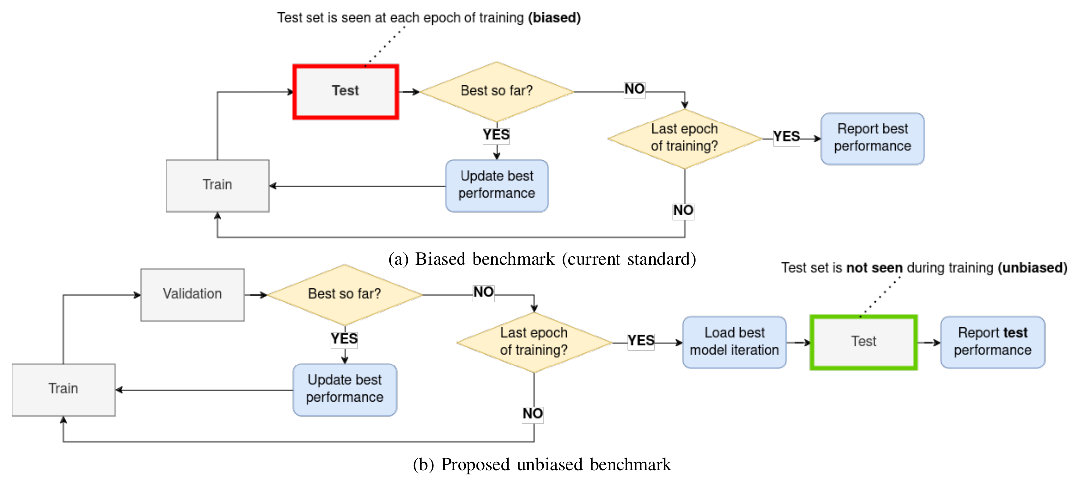
The loops in the two flowcharts look almost the same. The difference is the box inside the loop that does the “pick the best” job. In the upper chart it is Test, in a red box, consulted after every epoch; in the lower chart it becomes Validation, and Test moves outside the loop to run only once, at the end.
Both options keep the test set entirely out of the training process. The authors prefer the first, because people still want to see results on the four familiar datasets, O, C, I, and M.
How should the fifth dataset be chosen? The authors weighed four things: amount of data, attack types, number of subjects, and sample variation. In the end they picked two candidates:
| Dataset | Year | Subjects | Live | Attack | Attack types |
|---|---|---|---|---|---|
| CASIA | 2012 | 50 | 150 | 450 | Print, replay |
| Replay | 2012 | 50 | 200 | 1,000 | Print, replay |
| MSU | 2014 | 35 | 70 | 210 | Print, replay |
| Oulu | 2017 | 55 | 720 | 2,880 | Print, replay |
| SiW | 2018 | 165 | 1,320 | 3,300 | Print, replay |
| Rose-Youtu | 2018 | 20 | 897 | 1,601 | Print, replay, mask |
SiW and Rose-Youtu are comparable in scale to OULU-NPU and more recent, with variation in lighting, environment, and attacks; SiW also varies in pose and expression. Rose-Youtu includes paper-mask attacks, which the authors removed so that the test still contains only prints and replays, with no new attack types mixed in.
For models, the authors chose four. ImageNet-pretrained ResNet-18 and ResNet-50 serve as baselines, joined by SA-FAS and GAC-FAS, two methods with public code whose reruns come close to their original papers' results. The metrics remain HTER and AUC.
Discussion
First, Rerun the Original Benchmark
The authors first reran SA-FAS and GAC-FAS under the original benchmark, in which the test set doubles as the validation set, and also tested the weights released by the GAC-FAS authors. Even with the original code and the same data, the numbers still differed from the original papers. On OCI→M, for example, GAC-FAS reports 5.00% in its paper, the released weights also give 5.00%, and the authors' own retraining gives 7.92%; on OMI→C, the three numbers are 8.20%, 10.00%, and 12.22%.
With the same code, a single retraining can be off by several percentage points. In all the comparisons that follow, the authors set their own rerun numbers against their own rerun numbers.
Picking with a Validation Set Instead
The main results are in Table III. Below is an excerpt for SiW as the validation set. The left of each arrow is the original benchmark, and the right is validation on SiW, in HTER (%):
| Test dataset | SA-FAS | GAC-FAS |
|---|---|---|
| OULU-NPU | 12.13 → 13.81 | 10.52 → 7.91 |
| Replay-Attack | 9.00 → 21.50 | 5.00 → 8.55 |
| CASIA-FASD | 14.00 → 26.67 | 12.22 → 9.14 |
| MSU-MFSD | 11.43 → 11.43 | 7.92 → 7.31 |
SA-FAS rises from 9.00% to 21.50% on Replay-Attack and from 14.00% to 26.67% on CASIA-FASD, roughly doubling in both; on MSU-MFSD it stays the same.
GAC-FAS goes the opposite way. Three of the four improve, and its 7.91% on ICM→O is even lower than the 8.60% reported in its original paper. The authors list this as an unexpected finding and do not analyze the cause further. At the very least, once the benchmark changes, a single method's numbers need not all move in the same direction.
The two ResNet baselines also go their separate ways. With SiW validation, ResNet-18 gets worse in all four settings; OCM→I, for example, rises from 31.50% to 37.50%. ResNet-50 improves in two, with OCI→M falling from 32.08% to 25.42% and ICM→O from 33.33% to 32.78%, and the authors list it alongside GAC-FAS as an example of improvement.
Validation Sets Need Choosing Too
With Rose-Youtu as the validation set, all models generally do worse. SA-FAS on OMI→C, for example, scores 26.67% with SiW validation and 40.67% with Rose-Youtu validation. The same holds with Rose-Youtu as the test set; it is much harder than SiW. Training on O, C, and I with MSU-MFSD as the validation set, SA-FAS and GAC-FAS reach HTERs of 10.05% and 9.58% when tested on SiW, which become 25.18% and 32.74% when tested on Rose-Youtu. The same two models are still reasonably usable on one new dataset, and on another, the HTER climbs above 25%.
The authors also looked at the EER on the validation set and the HTER on the test set. Normally the validation score is better than the test score, which the authors say is consistent with experience in the machine learning literature. Experiments validated on Rose-Youtu, however, show the opposite trend. The authors think this may come from a domain gap between the validation and test data, and from this they speculate that SiW's domain is closer to the four test datasets than Rose-Youtu's.
This raises a new question. The test set is put away, but the choice of validation dataset also changes which epoch gets picked and the final score. The authors recommend trying both; if you can run only one, use SiW as the validation set and run the four settings ICM→S→O, OCM→S→I, OCI→S→M, and OMI→S→C.
Taking It into the Wild
Finally, the authors took SA-FAS and GAC-FAS, trained on OCIM, and tested them on WFAS. WFAS was built by crawling the web and has 1,383,246 images, 469,920 people, and 17 attack types, roughly 300 times the size of SiW. Its test labels are kept private, and APCER, BPCER, and ACER can be obtained only through the challenge platform.
Both methods land at ACERs between 28.62% and 32.54%, each winning in two of the four settings. The WFAS challenge winner scored 2.82%. The authors also trained GAC-FAS directly on the WFAS training set and took the model from the final iteration, for an ACER of 21.51%.
WFAS has many attack types that OCIM lacks, so this test examines cross-dataset and cross-attack-type generalization at the same time, a problem these methods were never designed to solve. Deployment, however, looks exactly like this.
Conclusion
The problem this paper sets out to solve is clear. The OCIM convention lets the test set be checked again and again during training, so the reported numbers look better than what deployment actually delivers. The authors' fix is simple, too. Add one dataset as a validation set, and look at the test set only after training ends.
Judging from the experiments, how large this bias is depends on the method. SA-FAS's HTER roughly doubles in two settings, while GAC-FAS mostly improves instead. So the ranking of “which is better” may itself change with the benchmark. The choice of validation set also affects the results; SiW and Rose-Youtu give very different numbers.
The limitations deserve a look as well. This is work in progress that reruns only two DG methods and two ResNet baselines, and the paper does not say how many random seeds each experiment used; the rerun numbers themselves already differ from the original papers. The authors give the location of their code in the paper and say it will be released after publication.
If you are putting a model into production, you can apply this approach to your own evaluation pipeline right away. Pick epochs and thresholds with data other than the test set, and leave the test set sealed until the very end.