[16.03] RARE

Automatic Rectification

Robust Scene Text Recognition with Automatic Rectification

---

After the introduction of CRNN, many issues were resolved, but it still struggled with recognizing irregular text.

Defining the Problem

Recognizing text in natural scenes is much harder than recognizing printed text. During recognition, text can often appear distorted, warped, occluded, or blurred.

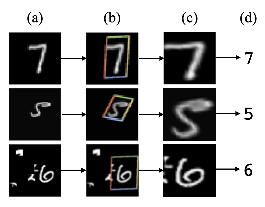
In this paper, the authors focus on addressing the problems of deformation and distortion. Remember that famous STN model from a while back?

• [15.06] Spatial Transformer Networks

  

Maybe we could design a model with automatic rectification functionality?

Solving the Problem

Spatial Transformer Network

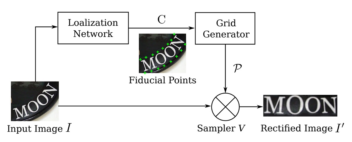
To alleviate the issue of recognizing irregular text, the automatic rectification functionality should be placed before the recognition module.

Here, the authors introduce a Spatial Transformer Network (STN) to rectify the input image.

The primary goal of the STN is to transform the input image $I$ into a rectified image $I'$ using a predicted Thin Plate Spline (TPS) transformation. This network predicts a set of control points through a localization network, calculates TPS transformation parameters from these points, and generates a sampling grid that is used to produce the rectified image $I'$ from the input image.

Localization Network

The localization network is responsible for locating $K$ control points. Its output is the coordinates of these control points in $x$ and $y$, denoted as:

$$C = [c_1, \dots, c_K] \in \mathbb{R}^{2 \times K}, c_k = [x_k, y_k]^\top$$

The coordinate system’s center is set at the center of the image, and the coordinate values range from $[-1, 1]$.

The network uses a convolutional neural network to regress the control points’ positions. The output layer consists of $2K$ nodes, using the tanh activation function to ensure the output values fall within the $(-1, 1)$ range.

The network is fully supervised by backpropagated gradients from the other parts of the STN, so no manual labeling of control point coordinates is required.

Grid Generator

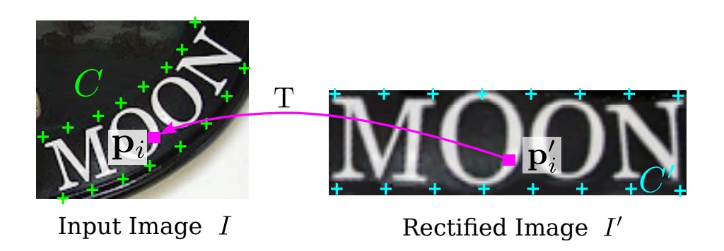
The authors define a set of "base" control points (as shown in the above image), which are then adjusted by the control points $C$ predicted by the localization network to obtain new control points $C^\prime$.

The grid generator estimates the TPS transformation parameters and produces the sampling grid. The TPS transformation parameters are represented by a matrix $T \in \mathbb{R}^{2 \times (K+3)}$, calculated as:

$$T = \left( \Delta_{C^\prime}^{-1} \begin{bmatrix} C^\top \\ 0^{3 \times 2} \end{bmatrix} \right)^\top$$

Here, $\Delta_{C^\prime} \in \mathbb{R}^{(K+3) \times (K+3)}$ is a matrix determined by the control points $C^\prime$, thus being a constant matrix.

The specific form of $\Delta_{C^\prime}$ is:

$$\Delta_{C^\prime} = \begin{bmatrix} 1 & (C^\prime)^{\top} & R \\ 0 & 0 & 1^{1 \times K} \\ 0 & 0 & C^\prime \end{bmatrix}$$

Where the element $r_{i,j}$ in the matrix $R$ is defined as:

$$r_{i,j} = d_{i,j}^2 \ln d_{i,j}^2,$$

Here, $d_{i,j}$ represents the Euclidean distance between the $i^{th}$ and $j^{th}$ control points $c^\prime_i$ and $c^\prime_j$.

The pixel grid on the rectified image $I'$ is denoted as $P' = \{p'_i\}_{i=1, \dots, N}$, where $p'_i = [x'_i, y'_i]^{\top}$ is the $x$ and $y$ coordinates of the $i^{th}$ pixel, and $N$ is the number of pixels in the image.

For each pixel $p'_i$ in $I'$, its corresponding pixel $p_i = [x_i, y_i]^{\top}$ in the input image $I$ is determined by the following transformation:

1. First, calculate the distance between $p'_i$ and the control points:

   $$r'_{i,k} = d_{i,k}^2 \ln d_{i,k}^2,$$

   Where $d_{i,k}$ is the Euclidean distance between $p'_i$ and the $k^{th}$ control point $c^\prime_k$.

2. Next, construct the augmented vector $\hat{p}'_i$:

   $$\hat{p}'_i = \left[ 1, x'_i, y'_i, r'_{i,1}, \dots, r'_{i,K} \right]^{\top}.$$

3. Finally, use the matrix operation below to map it to the point $p_i$ on the input image:

   $$p_i = T \hat{p}'_i.$$

By applying the above steps to all the pixels in the rectified image $I'$, a pixel grid $P = \{p_i\}_{i=1, \dots, N}$ on the input image $I$ is generated.

Since the matrix $T$ calculation and the transformation of points $p_i$ are differentiable, the grid generator can backpropagate gradients for model training.

tip

If you find the above explanation too technical, let’s simplify it:

Imagine we have a distorted image (perhaps due to the camera angle or other factors). We want to "flatten" or "correct" it, making its content orderly so that recognition becomes easier.

First, we select some "control points" on the image. These points can be important reference locations in the image, like corners or edges. We then calculate the relationships between these control points, using Euclidean distances. Based on these distances, we can determine how each pixel in the image should move or adjust to make the image flat.

The "flattening" process doesn’t move each pixel randomly but follows a set of rules and calculations to ensure the rectified image remains consistent and natural.

That’s what the matrix $T$ and those distance formulas are doing.

Sampler

The sampler uses bilinear interpolation to generate the rectified image $I'$ from the input image $I$ based on pixel values.

For each pixel $p'_i$ in the rectified image $I'$, its value is calculated through bilinear interpolation of the nearby pixels in the input image $I$.

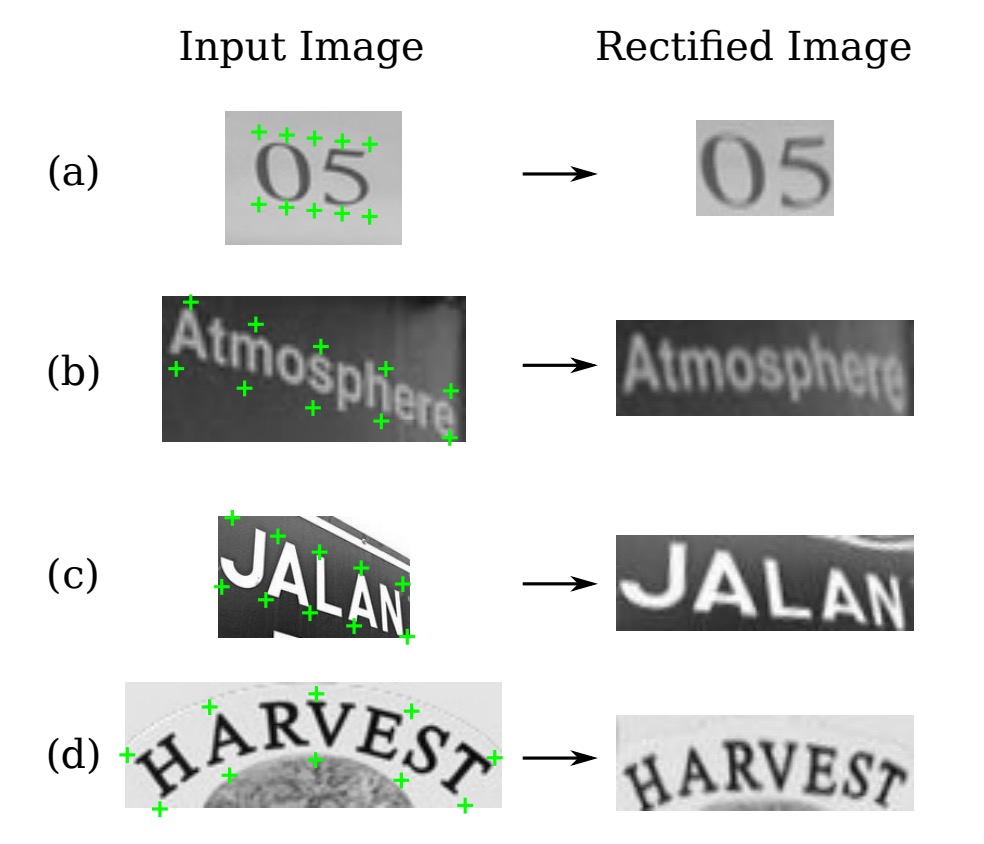
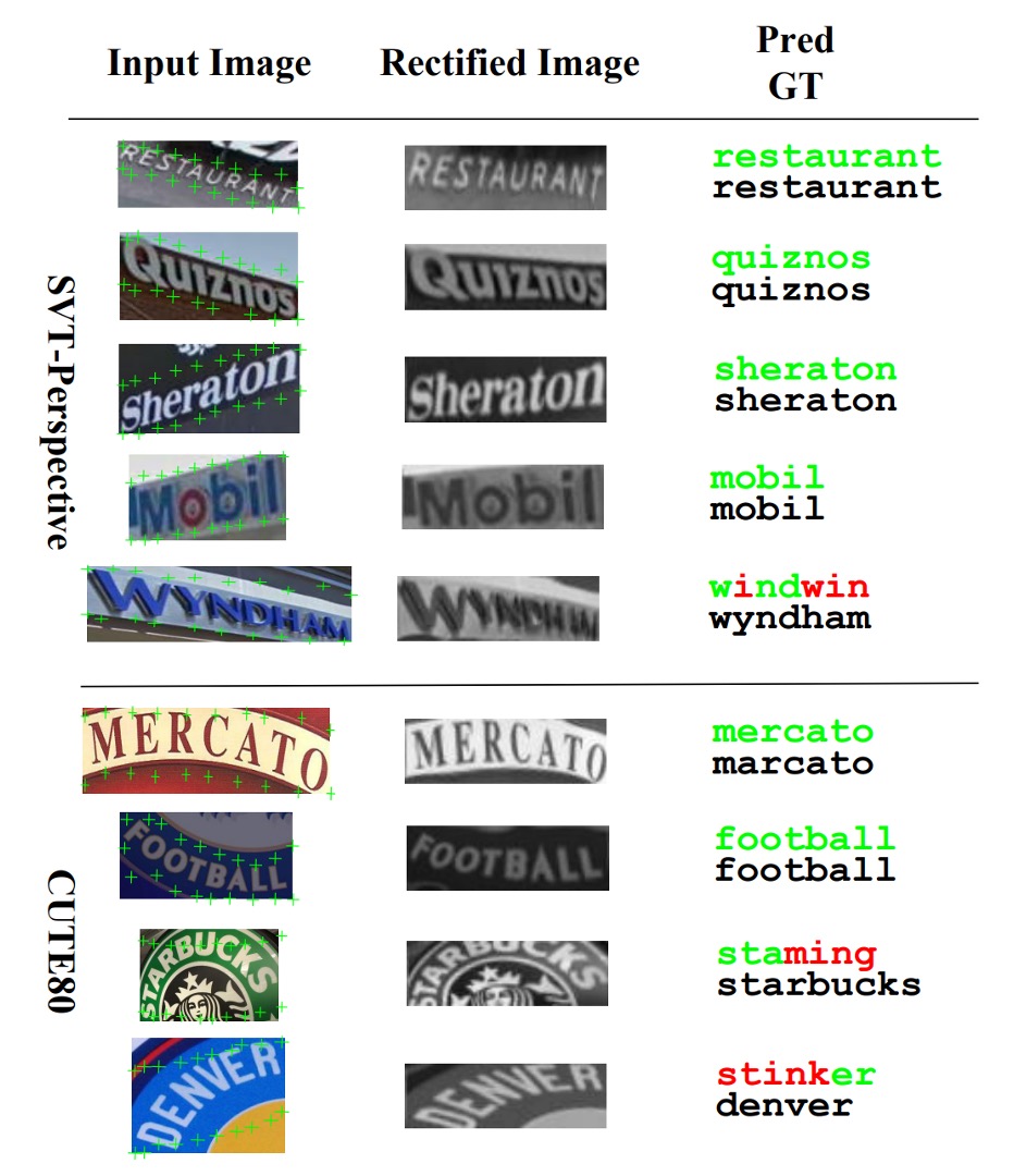
This process is also differentiable, allowing the entire model to backpropagate errors. The sampled result looks like the following image:

Encoder-Decoder

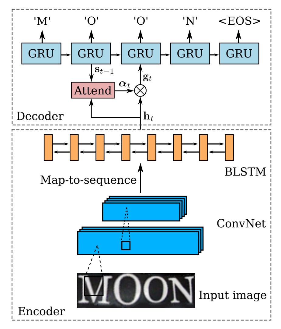
After completing the automatic correction of the image, we return to the familiar recognition process.

First, we have the encoder, where a CRNN model is used. This model uses a backbone network to convert the input image into a sequence of features, which are then fed into a BiLSTM network for sequence modeling.

Next comes the decoder. In the original CRNN model, the CTC algorithm was used for text decoding, but in this paper, the authors opted for a simpler method: using a GRU (Gated Recurrent Unit) for decoding.

tip

GRU and LSTM are similar architectures, but GRU has fewer parameters, which leads to faster training times.

For the decoding part, the authors integrated an attention mechanism. At each time step $t$, the decoder calculates an attention weight vector $\alpha_t \in \mathbb{R}^L$, where $L$ is the length of the input sequence.

The formula for calculating the attention weights is as follows:

$$\alpha_t = \text{Attend}(s_{t-1}, \alpha_{t-1}, h)$$

Where:

• $s_{t-1}$ is the hidden state of the GRU unit from the previous time step.
• $\alpha_{t-1}$ is the attention weight vector from the previous time step.
• $h$ is the encoder’s representation of the input sequence.

The Attend function calculates the current attention weight vector $\alpha_t$ based on the previous hidden state $s_{t-1}$ and the previous attention weights $\alpha_{t-1}$. Each element of this vector is non-negative, and the sum of all elements equals 1, representing the importance of each element in the input sequence for the current decoding step.

Once $\alpha_t$ is computed, the model generates a vector called the glimpse vector $g_t$, which is the weighted sum of the encoded representation $h$ of the input sequence.

The formula for the glimpse vector is:

$$g_t = \sum_{i=1}^{L} \alpha_{ti} h_i$$

Where:

• $\alpha_{ti}$ is the $i$-th element of the attention weight vector $\alpha_t$.
• $h_i$ is the encoded representation of the $i$-th element of the input sequence.

The glimpse vector $g_t$ represents the weighted sum of the parts of the input sequence that the model is currently focusing on.

Since $\alpha_t$ is a probability distribution (with all elements being non-negative and summing to 1), the glimpse vector $g_t$ is a weighted combination of the input sequence’s features. This allows the decoder to focus on different parts of the input sequence depending on the current decoding step.

After computing the glimpse vector $g_t$, the decoder uses the GRU’s recursive formula to update the hidden state $s_t$:

$$s_t = \text{GRU}(l_{t-1}, g_t, s_{t-1})$$

Where:

• $l_{t-1}$ is the label from the previous time step.
• During training, this is the actual label.
• During testing, this is the predicted label from the previous time step $\hat{l}_{t-1}$.
• $g_t$ is the glimpse vector calculated using the attention mechanism, representing the part of the input the model is focusing on.
• $s_{t-1}$ is the hidden state of the GRU from the previous time step.

The GRU unit updates the current hidden state $s_t$ based on the previous label $l_{t-1}$, the current glimpse vector $g_t$, and the previous hidden state $s_{t-1}$, encoding the relationship between the current step’s output and the input information.

At each time step, the decoder predicts the next output character based on the updated hidden state $s_t$. The output $\hat{y}_t$ is a probability distribution over all possible characters, including a special "End of Sequence" (EOS) symbol. Once the model predicts EOS, the sequence generation process is complete.

Dictionary-Assisted Recognition

The final output might still contain some errors. The authors use a dictionary to aid recognition. They compare the results with and without the dictionary.

When testing images with an associated dictionary, the model selects the word with the highest conditional posterior probability:

$$l^* = \arg \max_l \log \prod_{t=1}^{|l|} p(l_t | I; \theta).$$

When the dictionary is very large (e.g., a Hunspell dictionary containing over 50k words), checking each word’s probability can be computationally expensive. Therefore, the authors adopt a prefix tree for efficient approximate search, as shown below:

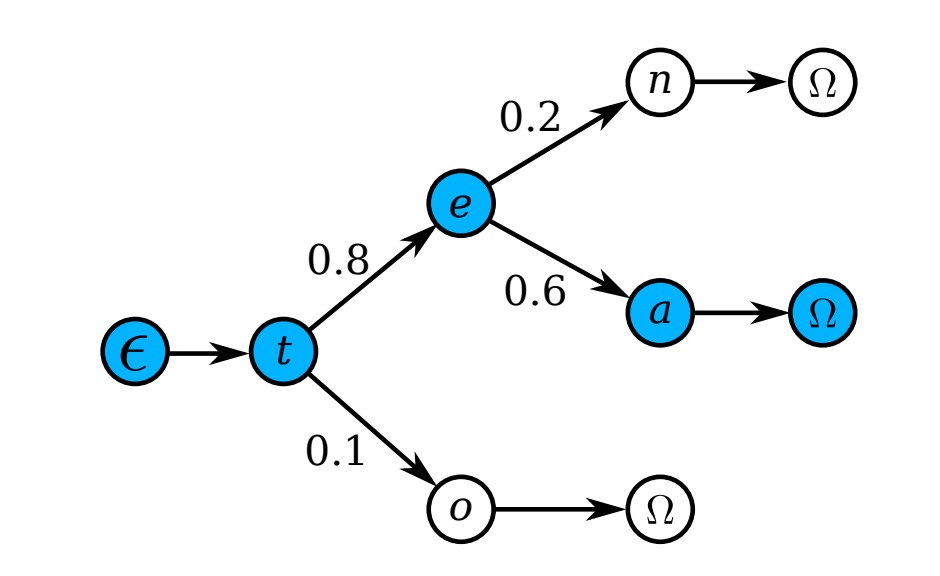
Each node represents a character, and the path from the root to the leaf represents a word.

During testing, starting from the root node, the highest posterior probability sub-node is selected at each step based on the model’s output distribution, continuing until reaching a leaf node. The corresponding path is the predicted word.

Since the tree's depth is the length of the longest word in the dictionary, this method is much more efficient than searching each word individually.

Model Training

The authors used a synthetic dataset released by Jaderberg et al. as training data for scene text recognition:

• Text Recognition Data: This dataset contains 8 million training images with corresponding annotated text. These images are generated by a synthetic engine and are highly realistic.

No additional data was used.

The batch size during training was set to 64, and the image size was adjusted to $100 \times 32$ during both training and testing. The STN's output size was also $100 \times 32$. The model processes approximately 160 samples per second and converged after 3 epochs, which took about 2 days.

Evaluation Metrics

The authors evaluated the model's performance using four common scene text recognition benchmark datasets:

1. ICDAR 2003 (IC03)

   • The test set contains 251 scene images with labeled text bounding boxes.
   • For fair comparison with previous works, text images containing non-alphanumeric characters or less than three characters are usually ignored. After filtering, 860 cropped text images remain for testing.
   • Each test image is accompanied by a 50-word lexicon (dictionary). Additionally, a full lexicon is provided, which merges the lexicons of all images for evaluation.

2. ICDAR 2013 (IC13)

   • The test set inherits and corrects part of the IC03 data, resulting in 1,015 cropped text images with accurate annotations.
   • Unlike IC03, IC13 does not provide a lexicon, so evaluations are done without dictionary assistance (i.e., in a no-dictionary setting).

3. IIIT 5K-Word (IIIT5k)

   • The test set contains 3,000 cropped text images collected from the web, covering a wider range of fonts and languages.
   • Each image comes with two lexicons: a small dictionary containing 50 words and a large dictionary containing 1,000 words for dictionary-assisted evaluation.

4. Street View Text (SVT)

   • The test set comprises 249 scene images from Google Street View, cropped into 647 text images.
   • Each text image is accompanied by a 50-word lexicon for dictionary-assisted evaluation.

Discussion

Comparison with Other Methods

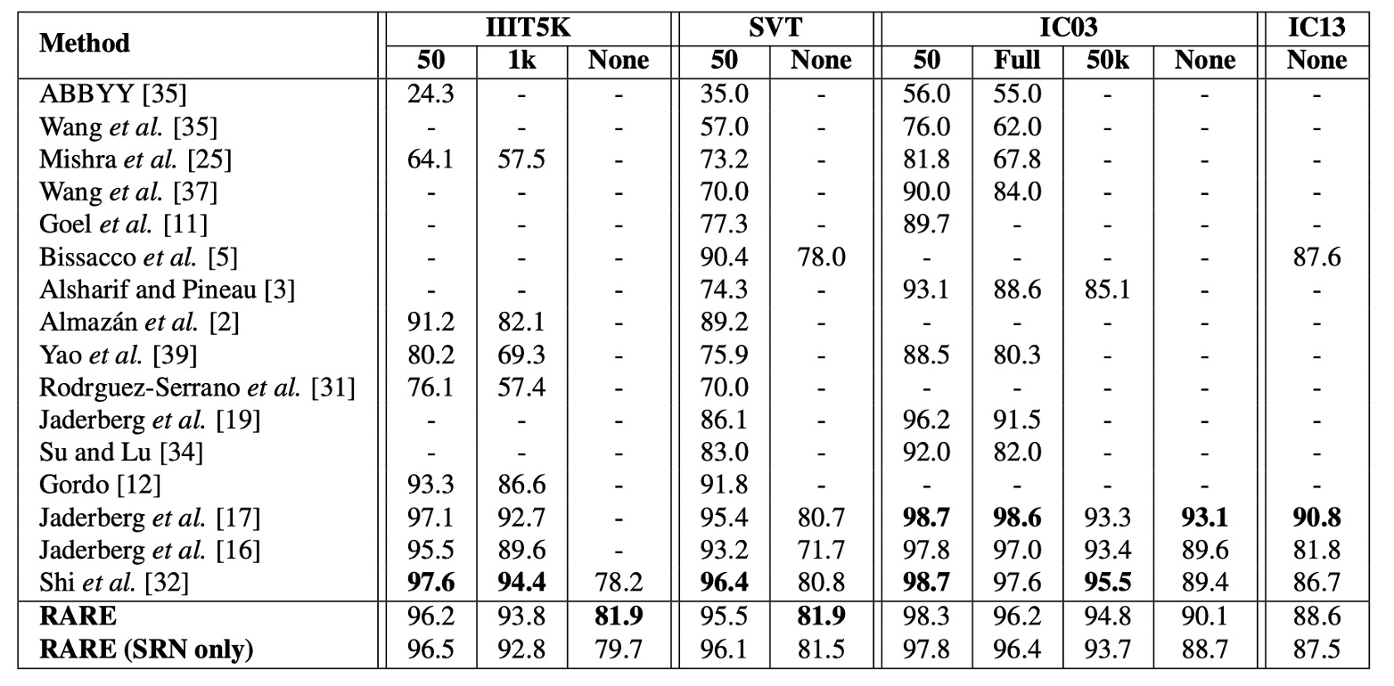
The table above shows the results of the model on the benchmark datasets, compared to other methods. In the "without dictionary assistance" task, the model outperforms all compared methods.

On the IIIT5K dataset, RARE improves performance by nearly 4 percentage points compared to CRNN【32】, showing a significant performance boost. This is because IIIT5K contains a large number of irregular texts, especially curved text, where RARE has an advantage in handling irregularities.

Although the model falls behind the method in【17】on some datasets, RARE is able to recognize random strings (such as phone numbers), while the model in【17】is limited to recognizing words within its 90k-word dictionary.

In the dictionary-assisted recognition task, RARE achieves comparable accuracy to【17】on IIIT5K, SVT, and IC03, and only slightly falls behind CRNN, demonstrating strong competitive performance even with dictionary assistance.

tip

At that time, it wasn't common to name your theoretical approach or method. Hence, we often see naming conventions based on the author's name, such as method 【17】 in the table, which refers to Jaderberg et al.'s paper:

• [14.12] Reading text in the wild with convolutional neural networks

Conclusion

This paper primarily addresses the problem of recognizing irregular text by introducing a differentiable Spatial Transformer Network (STN) module to automatically rectify irregular text and achieve end-to-end training, achieving good performance on several benchmark datasets.

The authors also pointed out that the model performs poorly on "extremely curved" text, possibly due to the lack of corresponding data types in the training set, which presents an opportunity for future improvements.

tip

Around 2020, we attempted to deploy this model, but encountered difficulties when converting it to ONNX format, mainly because ONNX did not support grid_sample or affine_grid_generator at that time.

We stopped paying attention to the model after that, but if you have successfully deployed it, feel free to share your experience with us.