Original paper
Quasi-Dense Similarity Learning for Multiple Object Tracking
- Publication
- CVPR 2021Conference
- First submitted to arXiv
- arXiv:2006.06664
Cite this paper · BibTeX
The citation identifies the linked source version. It cites the original paper and its authors.
@misc{multiobjecttrackingqdtrack2020,
  title = {{Quasi-Dense Similarity Learning for Multiple Object Tracking}},
  author = {Jiangmiao Pang and Linlu Qiu and Xia Li and Haofeng Chen and Qi Li and Trevor Darrell and Fisher Yu},
  year = {2020},
  eprint = {2006.06664},
  archivePrefix = {arXiv},
  url = {https://arxiv.org/abs/2006.06664}
}
By 2020, association in multi-object tracking relied mainly on position.
SORT uses IoU, CenterTrack predicts center-point displacements, and Tracktor has the detector's regression head push boxes into the next frame. As long as detection is accurate enough, the positional relationship between two adjacent frames is a very strong cue. Appearance features usually just lend a hand, used to recover targets that have disappeared for a while, and even then the search has to be limited to the neighborhood, because appearance features aren't reliable enough, and widening the range makes mistakes more likely.
But when people track objects, looks alone are often enough. Jiangmiao Pang of Zhejiang University, Fisher Yu of ETH Zürich, Trevor Darrell of UC Berkeley and colleagues argue that appearance features are unreliable because of how wastefully they're trained.
Defining the problem
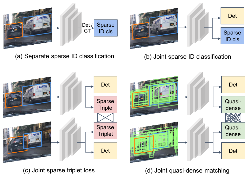
The methods for learning appearance features at the time fell roughly into these groups:
- Identity classification: treat each identity in the training set as a class, as in DeepSORT's re-ID model and the embedding branches that JDE and FairMOT add to their detectors. The bigger the dataset, the more classes, and the harder it is to scale.
- Triplet loss: each sample is compared with just one positive and one negative.
Either way, the only training samples are the ground-truth boxes, perhaps a dozen or so per image.
Yet a detector proposes hundreds of candidate regions on every image. Those close to a ground-truth box could serve as extra positives; those on the background are ready-made hard negatives. These regions were only ever used to train detection, and all of them were thrown away when learning appearance.
The authors want to use all of these candidate regions to learn appearance. If the feature space is learned well enough, association needs no position, motion or displacement prediction; just find the nearest neighbor in feature space.
Solving the problem
Quasi-dense sampling
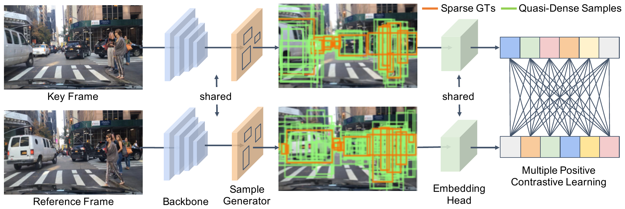
The authors define "dense matching" as matching candidate boxes at every pixel position; "quasi-dense" takes only the informative regions likely to contain objects, namely the proposals from the RPN.
The detector is a standard Faster R-CNN with FPN and a ResNet-50 backbone. Alongside the existing box classification and box regression heads, a lightweight embedding head (4 convolutional layers plus 1 fully connected layer) is added in parallel, outputting a 256-dimensional feature for each proposal.
During training, each step takes one key frame and then picks a reference frame at random from within 3 frames before or after it. Each of the two images goes through the RPN to get proposals:
- A proposal with an IoU above 0.7 with some real object counts as a sample of that object; below 0.3, it counts as background.
- If a proposal in the key frame and a proposal in the reference frame belong to the same object, the pair is a positive; otherwise it's a negative.
From the key frame, 128 proposals are taken as training samples, and from the reference frame, 256 as contrastive targets, half positive and half negative. Each training sample is compared with all 256 targets in the reference frame.
A contrastive loss with multiple positives
With only one positive, the standard softmax cross-entropy works. Let be the training sample's feature, the positive and the negatives:
But after quasi-dense sampling, a training sample has several positives in the reference frame, since every proposal near the same object counts. Simply summing the positives in the numerator would count each negative several times while counting the positives only once.
The authors first rewrite the equation above as
and then accumulate over the positives as well:
This way, every positive-negative pair is compared exactly once, on an equal footing.
On top of that, an auxiliary L2 loss constrains the cosine similarity of the features:
for positive pairs and for negative pairs. The authors explain that this loss serves to constrain the magnitude of the logits and the cosine similarity; it doesn't directly improve results.
The overall loss is
with and . The appendix mentions that performance drops when goes above 0.5.
Association by appearance alone
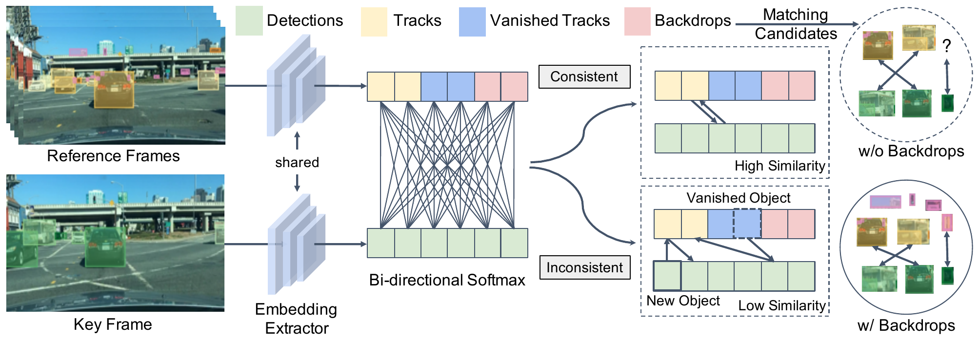
At inference time, association uses no position at all. But finding nearest neighbors by features alone gets messy when a detection has no corresponding track at all (a new object, a false positive), or when there are several candidates that all look alike. The authors handle this with three designs.
Bi-directional softmax. The current frame has detections with features ; there are matching candidates with features . Their similarity is the average of softmaxes taken in both directions:
The first term asks "among all candidates, which one does detection look most like?" and the second asks "among all detections, which one does candidate look most like?" The score is high only when the two are each other's nearest neighbors. A newly appearing object has no true counterpart among the candidates, so it's hard for both directions to score high at once, and it naturally doesn't get matched.
Keeping backdrops. Earlier methods simply threw away detections that didn't match any track. The authors argue that although these boxes are mostly false positives, the false positives in the next frame will very likely look the same. Keep them for one frame as matching candidates, and the next frame's false positives will match these backdrops instead of being forced onto real tracks.
Cross-class duplicate removal. Ordinary detectors only apply non-maximum suppression within each class, so the same location may get both a "pedestrian" box and a "rider" box, each with nearly identical features. The authors run one more round of cross-class non-maximum suppression before association, with a threshold of 0.7 for high-confidence boxes and 0.3 for low-confidence ones.
The rest are the usual thresholds. Only a detection with confidence above 0.8 starts a new track, vanished tracks are kept for 10 frames, track features are updated with a momentum of 0.8, and only objects of the same class can be matched with each other.
Discussion
Which designs help
| Training | Similarity | D.R. | BD | MOTA | IDF1 | Ped. MOTA | Ped. IDF1 |
|---|---|---|---|---|---|---|---|
| Sparse | cosine | 60.4 | 63.0 | 37.6 | 49.7 | ||
| Quasi-dense, single positive | cosine | 61.5 | 66.8 | 40.5 | 52.7 | ||
| Quasi-dense, multi-positive | cosine | 62.5 | 67.8 | 44.0 | 54.3 | ||
| Quasi-dense, multi-positive | bi-softmax | 62.9 | 70.0 | 45.5 | 58.8 | ||
| Quasi-dense, multi-positive | bi-softmax | ✓ | 63.2 | 70.1 | 45.5 | 58.3 | |
| Quasi-dense, multi-positive | bi-softmax | ✓ | ✓ | 63.5 | 71.5 | 46.7 | 60.2 |
Compiled from Table 4 of the paper, BDD100K tracking validation set. D.R. = cross-class duplicate removal; BD = backdrops.
The ablations are run on the BDD100K validation set. This is a dashcam dataset with 8 classes, much larger than MOT17.
Going from sparse to quasi-dense raises IDF1 from 63.0 to 67.8. Of that, simply adding more negatives while still using the single-positive loss contributes 3.8 points, about 80% of this improvement. The more contrastive targets there are, even if most of them are negatives, the better the features get learned. The multi-positive loss adds another point.
On the inference side, the bi-directional softmax adds another 2.2 points of IDF1, and 4.5 points for the pedestrian class. Duplicate removal and backdrops add 1.5 more. From start to finish, IDF1 improves by 8.5 points in total, and ID switches drop by 30%. The pedestrian class shows it most clearly, with MOTA and IDF1 up 9.1 and 10.5 points respectively.
Is position still any use?
| Appearance | IoU | Motion | Regression | mMOTA | mIDF1 |
|---|---|---|---|---|---|
| ✓ | 26.3 | 36.0 | |||
| ✓ | ✓ | 27.7 | 38.5 | ||
| ✓ | ✓ | 28.6 | 39.3 | ||
| ✓ | 36.6 | 50.8 | |||
| ✓ | ✓ | 36.3 | 49.8 | ||
| ✓ | ✓ | ✓ | 36.4 | 49.9 | |
| ✓ | ✓ | ✓ | 36.4 | 50.1 |
Compiled from Table 5 of the paper, BDD100K tracking validation set; mMOTA and mIDF1 are averages over the 8 classes.
Following Tracktor's approach, the authors add positional cues such as IoU, a motion model and box regression on top of the same detector.
Without appearance features, every additional positional cue improves results. But once the appearance features learned by quasi-dense sampling are in place, adding any positional cue doesn't help and even lowers the numbers slightly. The best result comes from appearance alone.
If appearance features are learned well enough, positional cues aren't needed; that's the paper's core claim. This result is on BDD100K, though. Its tracking annotations are at 5 frames per second, and the camera is mounted on a moving car, so an object's position and size can change a lot between two adjacent annotated frames, and positional cues aren't all that reliable there in the first place.
The benchmarks
QDTrack reports results on four benchmarks and uses no extra training data apart from COCO pretraining.
- MOT17 (private detections): a MOTA of 68.7 and IDF1 of 66.3 at 20.3 frames per second. That's 0.9 and 1.6 points above CenterTrack at the time, and CenterTrack used extra data. Its 3,378 ID switches are more than CenterTrack's 3,039; the authors explain that its recall is higher, with 14,000 fewer FN, and the more tracks it follows, the more chances there are to switch IDs.
- BDD100K: on the test set, an mMOTA of 35.5 and mIDF1 of 52.3, 9.2 and 7.6 points above the official baseline, and better than the winner of the 2020 BDD100K tracking challenge.
- Waymo: a MOTA of 55.6 for the vehicle class on the validation set, 10.7 points above RetinaTrack. With ResNet-101 and deformable convolutions, its test-set results are on par with the winner of the 2020 Waymo 2D tracking challenge, as a single model.
- TAO: this dataset has hundreds of classes with a severe long-tail distribution. Overall AP50 is only 2 to 3 points above the baseline, but for pedestrians, a common class, it's 38.6 vs. 18.5.
Detection is the bottleneck
Two oracle experiments in the appendix are well worth a look.
Replacing the detections with ground-truth boxes and then associating with QDTrack's features gives an average IDF1 of 88.8 over the 8 classes, 38 points higher than before. Conversely, keeping the detections as they are and associating with the true tracking labels raises mIDF1 by only 4.3 points.
In other words, on BDD100K, QDTrack's association is already close to its ceiling, and most of the error comes from detection. The failure cases say the same. Most of what's missed is very small or squeezed-in objects, and the false positives are people in mirrors or on billboards. Another case is class flipping: when a bicycle is occluded, for example, a "rider" gets detected as a "pedestrian," and since QDTrack only allows matches within the same class, the ID breaks.
What came after
The conclusion that "appearance alone is enough" was later re-examined on MOT17. On the MOT17 half validation set, ByteTrack added Kalman-filter motion cues to QDTrack's re-ID similarity and then applied its own BYTE association. MOTA went from 67.3 to 67.7, IDF1 rose from 67.8 to 72.0, and ID switches fell from 377 to 281. In surveillance footage, pedestrians walk slowly and steadily, and motion cues are still very useful there.
DanceTrack sits at the other extreme. There, the dancers dress alike and appearance is hard to tell apart, and in their own association experiments the DanceTrack authors found that simply adding appearance matching made things worse. Yet in the same paper, QDTrack retrained with a YOLOX detector reached a HOTA of 54.2, higher than ByteTrack's 47.7, and its association accuracy, AssA, was also 36.8 vs. 32.1. Features learned quasi-densely can still pick up some differences in scenes where everyone looks almost the same.
Conclusion
What QDTrack replaces is the sampling used to learn appearance features. Instead of just a dozen or so ground-truth boxes, all of the hundreds of proposals are compared against each other, paired with a contrastive loss that treats multiple positives fairly.
At inference time, only appearance is left, plus a few simple rules: the bi-directional softmax, backdrops kept for one frame, and cross-class duplicate removal. No Kalman filter, no IoU, and on BDD100K, adding positional cues even made things slightly worse.
The backdrop trick is especially fun. Most trackers are busy finding ways to throw false positives away; QDTrack keeps them around, so the next frame's false positives have somewhere to go.