Original paper
Simple Online and Realtime Tracking
- Publication
- ICIP 2016Conference
- First submitted to arXiv
- arXiv:1602.00763
Cite this paper · BibTeX
The citation identifies the linked source version. It cites the original paper and its authors.
@misc{multiobjecttrackingsort2016,
  title = {{Simple Online and Realtime Tracking}},
  author = {Alex Bewley and Zongyuan Ge and Lionel Ott and Fabio Ramos and Ben Upcroft},
  year = {2016},
  eprint = {1602.00763},
  archivePrefix = {arXiv},
  url = {https://arxiv.org/abs/1602.00763}
}
In 2015, MOTChallenge went live. The benchmark put multi-object tracking videos, annotations, public detections and evaluation code in one place, and people could finally compare trackers on the same leaderboard.
The top of that leaderboard was crowded with elaborate systems. Old methods from radar tracking, such as Multiple Hypothesis Tracking (MHT) and Joint Probabilistic Data Association (JPDA), were brought back out and paired with appearance models, online learning and all kinds of rules for handling occlusion. Accuracy did go up, but speed often dropped to one or two frames per second.
Alex Bewley and colleagues at Queensland University of Technology looked at this leaderboard and noticed two things. First, the top-ranked tracker happened to be the only method that did not use the official ACF detections. Second, the few most accurate methods were all too slow to run in real time.
If detection quality is the real bottleneck, does the tracker need to be this complicated?
This paper wants to find out how simple multi-object tracking can get, and how well it can still do.
Defining the problem
The input to multi-object tracking (MOT) is a video. The output is a box for every object in every frame, plus an ID that stays the same across frames.
The mainstream approach is called tracking-by-detection. A detector first finds all the boxes in each frame independently, and a tracker then strings those boxes into tracks. The detector only cares about "who is in this frame"; the tracker has to answer "which box in the previous frame is this one?" The latter is the data association problem.
This paper adds one more constraint: the tracker must be online. In other words, when it processes frame , it can only see frame and what came before, and it has to assign IDs on the spot. The other family, batch methods, can watch the whole video first and then go back and optimize globally. They usually do better, but they can't be used in settings such as self-driving cars or robots, which have to react in real time.
Here is what the leaderboard looked like at the time:
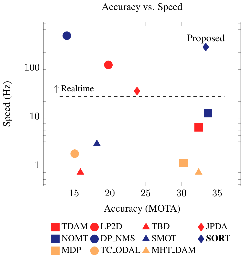
Accuracy runs along the horizontal axis and speed up the vertical axis, so further up and to the right is better. The bottom right holds methods that are accurate but slow, the top left methods that are fast but inaccurate, and the top right used to be empty.
Citing Occam's razor, the authors made a few extreme trade-offs for their tracker:
- Box position and size only. Apart from the detector, no appearance features are extracted at all; motion estimation and data association look only at boxes.
- No occlusion handling. The authors argue that short- and long-term occlusions rarely occur in this dataset, and that writing dedicated mechanisms for them would only make the system more complex. (MOT20 and DanceTrack, which came later, would probably both disagree with that "rarely.")
- No re-identification. An object that leaves the frame and comes back is treated as a new object. The authors' reasoning is that re-identification adds considerable computational overhead and gets in the way of real-time applications.
All that's left to get right is matching between two adjacent frames.
Solving the problem
SORT has four parts: detection, state estimation, data association, and the creation and deletion of tracks.
The detector
The authors use Faster R-CNN and compare two backbones, the shallower ZF and the deeper VGG16. The weights are the default parameters trained on PASCAL VOC, with no retraining for pedestrians; the output keeps only the "person" class, and only when its probability is above 50%.
This step looks mundane, yet it's the most important experimental variable in the whole paper. We'll come back to it in the discussion.
The state of each target
Each tracked object is described by a seven-dimensional vector:
is the pixel coordinate of the box center, is the box area, is the aspect ratio, and the last three entries are the velocities of the first three. The aspect ratio has no velocity term; the authors assume it doesn't change.
The motion model is a constant-velocity model: every frame, the velocity is added to the position, and the velocity stays the same. The official code writes this as a state transition matrix , plus an observation matrix that takes only the first four entries:
The first three rows of say "new position = old position + velocity"; says the detector can see directly but can't see velocity. The velocity has to be inferred by the Kalman filter from observations over several consecutive frames.
Every frame, the Kalman filter does two things. The first step is prediction: the motion model pushes the state forward one frame, and the uncertainty grows along with it:
The second step is the update. If a detection box is assigned to the track in this frame, the detection is used to correct the prediction:
is the state covariance, which says how unsure the filter is about itself; is the noise of the motion model, and the noise of the detection boxes. The Kalman gain decides whether to trust the prediction or the detection: the more uncertain the prediction (large ), the more it listens to the detection; the less reliable the detection (large ), the more it listens to the prediction.
If no detection box is assigned to the track in this frame, it only predicts and skips the update.
How matching works
At the start of each frame, every existing track first makes a prediction, which gives the box where it "should" appear in this frame. Then the intersection over union (IoU) between every detection box and every predicted box is computed and laid out as a matrix.
Matching has to be one-to-one: a detection box goes to at most one track, and a track takes at most one detection box. Maximizing the total IoU under this constraint is the classic assignment problem, and the Hungarian algorithm finds the optimal solution.
Why not just pair up whatever has the highest IoU? Let's look at a small example.
Suppose there are two tracks, A and B, and two detection boxes, 1 and 2, with this IoU matrix:
| Detection 1 | Detection 2 | |
|---|---|---|
| Track A | 0.60 | 0.50 |
| Track B | 0.55 | 0.00 |
With a greedy approach, you first take the largest value in the table, 0.60, and give detection 1 to A. That leaves B with only detection 2, at an IoU of 0, so no match. B loses its observation in this frame, detection 2 is treated as a new object, and the total IoU is 0.60.
The Hungarian algorithm looks at the whole picture. A takes detection 2 (0.50), B takes detection 1 (0.55), the total IoU is 1.05, and both tracks get a match. When two people walk side by side with overlapping boxes, this situation comes up all the time.
Once matching is done, any pair with an IoU below the threshold is broken up, so that two boxes that don't really overlap aren't forced into a pair. The official code uses a threshold of 0.3.
The authors also noticed a side benefit of IoU. When one person walks in front of another, the detector usually boxes only the person in front. That box is closer in size to the predicted box of the person in front, so IoU tends to give it to them. The occluded person gets no detection box, their state is only predicted, and it isn't dragged off by a wrong observation. Brief crossings get through this way, without any occlusion-handling rules at all.
Birth and death of tracks
If a detection box has an IoU below with every predicted box, it's treated as a newly appeared object, and a new track is created. The position is taken directly from the detection box, the velocity is set to zero, and the velocity covariance is set very large, meaning it's not yet known which way the object is heading.
A new track first goes through a probation period and only counts after several consecutive successful matches, which filters out the false positives the detector occasionally throws up. The paper doesn't give the number; min_hits in the official code is 3.
The deletion rule is even blunter. A track that goes consecutive frames without a detection box is deleted. The authors set to 1 in all experiments, for two reasons: the constant-velocity model predicts poorly to begin with, so leaving a track alone only lets it drift further away; and this paper only handles matching between adjacent frames, with re-identification out of scope.
If an object is occluded for a while and then reappears, it gets a new ID.
Discussion
The authors evaluate on MOTChallenge 2015 (MOT15). To tune the Kalman filter's initial covariance, and , they use the training and validation split from the MDP paper.
Two metrics are worth knowing first:
- MOTA (Multi-Object Tracking Accuracy): add up three kinds of errors, missed detections (FN), false positives (FP) and ID switches, divide by the total number of ground-truth boxes, and subtract the result from 1. All three errors count equally, but the first two usually outnumber ID switches by one or two orders of magnitude, so MOTA mostly reflects detection quality.
- ID sw: how many times the ID assigned to a ground-truth track changes, a direct measure of how well matching is done.
Swapping the detector
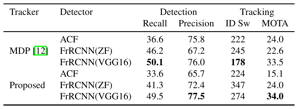
On the validation set, this table pairs each of the two trackers with three detectors. MDP was an online tracker that performed very well at the time, with a learned decision process; SORT is this paper's method.
Start with SORT's three rows. Switching the detector from ACF to FrRCNN(VGG16) raises MOTA from 15.1 to 34.0, a gap of 18.9 points. That gap is what the abstract means when it says changing the detector improves tracking by up to 18.9%. The tracking algorithm didn't change at all.
Now look at MDP. With FrRCNN(ZF), recall rises from 36.6 to 46.2, yet MOTA drops from 24.0 to 22.6. The problem is precision. ZF's precision falls from 75.8 to 67.2, false positives go up, and MOTA is docked for them too. A detector that "finds more" isn't always better for tracking; false positives come at a price as well.
With their best detector, the two trackers reach a MOTA of 33.5 and 34.0, a very small difference. The gap that detectors create is much larger than the gap between trackers.
The MOT15 test set
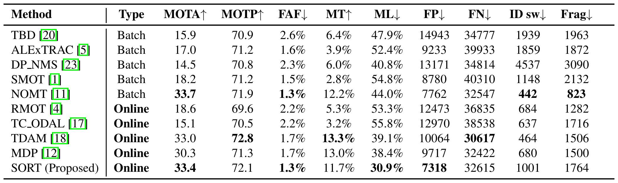
The test set has 11 sequences. The ground truth isn't public, and results are computed by the official server.
SORT's MOTA is 33.4, the highest among online methods and almost the same as NOMT (33.7), which gets to peek a few frames into the future. Its 7318 false positives are the fewest in the table, and its share of mostly lost tracks (ML), 30.9%, is also the lowest.
The ID switch column doesn't look so good, though. SORT has 1001, while MDP has 680, TDAM 464 and NOMT just 442. That's the price of and of using no appearance information: an object occluded for more than a frame or two comes back with a different ID. The number of track fragmentations (Frag), 1764, is on the high side too.
MOTA is high because detection is good; ID switches are many because matching is so simple. Put these two columns side by side, and SORT's strengths and weaknesses are plain to see.
Speed
The tracking part runs at 260 Hz on a single core of a 2.5GHz Intel i7, under 4 milliseconds per frame and more than 20 times faster than the other methods in the table.
That number only counts tracking, though, not detection. The FrRCNN(VGG16) that SORT uses runs at about 5 frames per second on the GPU used in the original Faster R-CNN paper. For the whole system to run in real time, the bottleneck is really the detector. This doesn't affect the paper's argument. What it sets out to show is that the tracking step can take almost no time, leaving the compute budget for the detector.
What came after
The official code's README says that SORT was the best-ranked open-source tracker on MOT15 when it was published, and it also notes that a large part of SORT's accuracy is down to the detections. The code itself is under three hundred lines, and it quickly became the default baseline in all kinds of projects.
Its parameters scattered along with it. Across different ports, max_age is 1 in some and 30 in others, and min_hits and the IoU threshold get their own tweaks. Before comparing against someone else's SORT numbers, check which settings they used.
In their conclusion, the authors write that a simple framework makes a good baseline, letting new methods concentrate on long-term occlusion and re-identification, and that in the future they plan to couple detection and tracking more tightly. A year later, DeepSORT, from Wojke, Bewley and colleagues, added appearance features back onto this skeleton. Methods such as JDE, FairMOT and CenterTrack, which put detection and tracking into the same network, took another path.
Conclusion
A Kalman filter, IoU and the Hungarian algorithm, three things straight out of the textbook, were enough for SORT to reach the highest MOTA among online methods on MOT15, with tracking itself taking under 4 milliseconds per frame. The most convincing numbers in the paper come from swapping the detector, which lifts MOTA from 15.1 to 34.0, while two trackers paired with the same good detector differ by just 0.5 points.
If you're building a new tracking system, get SORT running as a baseline first, then swap in a better detector and see how much the score moves. Only the gap that's left over is for the tracking algorithm to close.
Five years later, ByteTrack took first place on MOT17, and its association was still a Kalman filter plus IoU. It just picked up a few more low-score boxes.