Original paper
Essentially No Barriers in Neural Network Energy Landscape
- Publication
- ICML 2018Conference
- First submitted to arXiv
- arXiv:1803.00885
Cite this paper · BibTeX
The citation identifies the linked source version. It cites the original paper and its authors.
@misc{modelmergingnobarriers2018,
  title = {{Essentially No Barriers in Neural Network Energy Landscape}},
  author = {Felix Draxler and Kambis Veschgini and Manfred Salmhofer and Fred A. Hamprecht},
  year = {2018},
  eprint = {1803.00885},
  archivePrefix = {arXiv},
  url = {https://arxiv.org/abs/1803.00885}
}
When people talk about the loss landscape of a neural network, the most common picture is a landscape of separate valleys.
Training rolls downhill from some starting point and finally comes to rest at the bottom of some valley. Valley floors can be wide or narrow, and the wide ones supposedly generalize better. Different random seeds roll into different valleys, separated from one another by ridges. Draw a straight line between the weights at two valley floors and the loss along it first rises and then falls; plenty of people have measured exactly this.
Draxler, Veschgini, Salmhofer and Hamprecht at Heidelberg University saw the picture differently. The authors span an image processing lab and an institute for theoretical physics. They borrowed a tool for finding reaction paths from molecular statistical mechanics to see whether a route between two valley floors could avoid climbing over the mountains.
The answer was unexpected. For ResNets and DenseNets on CIFAR, the paths they found are almost flat.
At almost the same time, Garipov et al.'s mode connectivity independently arrived at the same observation. The two papers find their paths in completely different ways.
Defining the problem
Fix the architecture and the training data, and the loss is simply a function of the parameters . Take two parameter sets, and , each trained to convergence. We want a continuous path from to whose highest loss along the way is as low as possible:
This path is called the minimum energy path (MEP), and its highest point is the true saddle point between the two minima.
The authors use “loss” and “energy” as synonyms, a habit from physics. Valley floors in the loss landscape are stable states, and saddle points are the barriers that must be crossed to get from one state to another.
In two dimensions you can draw the grid and find the MEP with dynamic programming. Network parameters, however, easily number in the millions, so the only option is to start from an initial path and bend it toward low ground bit by bit using local information. The path found is not necessarily the exact MEP, and its highest point can serve only as an upper bound on the saddle-point energy.
So the paper's logic runs like this. As long as we can find a path whose highest point is very low, we have shown that the barrier between the two minima is no higher than that value.
Solving the problem
Pivots strung on springs
First, discretize the path. pivots form a chain with both ends fixed at the two minima, and .
The most intuitive approach is to connect the pivots with springs and minimize
The first term pulls every point toward low ground; the second keeps the points spaced apart.
The trouble is the spring constant . If is too small, the pivots slide downhill and the high-loss region ends up sparsely covered, even though the highest point is exactly what we most want to measure accurately. If is too large, the spring energy grows with the square of the total path length, and the whole chain is pulled taut, cutting corners and missing the true saddle point.
Nudged Elastic Band
NEB (Nudged Elastic Band) resolves this dilemma with a simple modification. It separates the two forces and keeps only the direction in which each one is useful:
Let be the local tangent direction at pivot :
The loss force keeps only its component perpendicular to the path, which pushes the path toward low ground; the spring force keeps only its component parallel to the path, which spaces the points evenly. That way, points on high ground do not slide down along the path, and the springs do not pull the path straight.
The choice of tangent matters too. points toward whichever of the two neighbors has the higher loss. This choice keeps kinks out of the path and gives a better approximation near the saddle point.
The authors go one step further in their implementation. They could not find a that worked well across different loss landscapes and different numbers of pivots, so they set the spring force to zero altogether. Instead, each iteration first redistributes the pivots evenly along the path and then applies the perpendicular loss force. In the literature this variant is also called the string method.
Walking through a two-dimensional example
A neural network has far too many parameters to draw. Let's switch to a two-dimensional landscape to see what NEB does:
The first term makes the loss zero on the unit circle; the second tilts the circle slightly, making and the two minima. The straight line between them passes through the origin, where the loss is 1; going around the circle, the highest point is only about 0.1.
import numpy as np

def loss(p):
    x, y = p[..., 0], p[..., 1]
    return (x**2 + y**2 - 1) ** 2 + 0.1 * y**2

def grad(p):
    x, y = p[..., 0], p[..., 1]
    r = x**2 + y**2 - 1
    return np.stack([4 * r * x, 4 * r * y + 0.2 * y], axis=-1)

def redistribute(path):
    seg = np.linalg.norm(np.diff(path, axis=0), axis=1)
    s = np.concatenate([[0], np.cumsum(seg)])
    t = np.linspace(0, s[-1], len(path))
    return np.stack([np.interp(t, s, path[:, d]) for d in range(2)], axis=1)

a, b = np.array([-1.0, 0.0]), np.array([1.0, 0.0])
path = np.linspace(a, b, 12)               # start: 12 pivots on the straight line
path[1:-1, 1] += 0.05                      # a small nudge so the path does not sit on the perfectly symmetric saddle
line_max = loss(np.linspace(a, b, 201)).max()

for step in range(2000):
    path = redistribute(path)              # the authors' approach: no springs, re-space evenly every iteration
    for i in range(1, len(path) - 1):
        lo, hi = path[i - 1], path[i + 1]
        tau = (hi - path[i]) if loss(hi) > loss(lo) else (path[i] - lo)
        tau /= np.linalg.norm(tau)
        g = grad(path[i])
        f_perp = -(g - (g @ tau) * tau)    # keep only the loss force perpendicular to the path
        path[i] = path[i] + 0.05 * f_perp

fine = np.concatenate([np.linspace(p, q, 20, endpoint=False) for p, q in zip(path[:-1], path[1:])] + [path[-1:]])
print(f"Highest loss on the straight line: {line_max:.3f}")
print(f"Highest loss on the NEB path: {loss(fine).max():.3f}")
x, y = fine[loss(fine).argmax()] + 0.0
print(f"Location of the highest point: ({x:.2f}, {y:.2f})")
Highest loss on the straight line: 1.000
Highest loss on the NEB path: 0.098
Location of the highest point: (-0.00, 0.96)
The barrier on the straight line is 1.0. NEB pushes the middle pivots up to near the circle, and the barrier drops to 0.098. That value is the saddle-point energy of this landscape. Minimizing along puts the saddle point at , .
The line that sets tau implements the rule described above, pointing toward the neighbor with the higher loss. If you replace f_perp with the full -g, the middle points slide along the circle toward the two ends and end up crowded near the two valley floors, leaving no point at all to measure the highest part of the path.
AutoNEB and the minimum spanning tree
In a space with millions of dimensions, nobody knows at the start how many pivots are needed. AutoNEB first runs a few rounds of NEB with a small number of pivots and then inspects the path. Wherever the loss between two adjacent pivots exceeds the estimate from linear interpolation between them by more than 20% of “the energy difference across the whole path,” it inserts a new pivot there. Nine extra points are evaluated between every pair of adjacent pivots to catch peaks of this kind that would otherwise be missed.
AutoNEB can still get stuck on a local minimum energy path and report a saddle that is too high. The authors handle this with an inequality. Given a path from A to B and one from B to C, joining the two gives a path from A to C, so
This is an ultrametric property. With it, as long as all the minima are linked into a graph by known paths, every pair of minima has an upper bound on its barrier; and if one path is too high, it can be replaced by a detour through other paths.
The authors therefore turn the problem into finding a minimum spanning tree. They first connect the first minimum to every other minimum, then repeatedly pick the highest edge in the tree and use AutoNEB to try to find a lower path between the two subtrees on either side of it. If a lower path turns up, it replaces the edge; if not, the edge goes back in. This continues until every pair has been tried or the compute budget runs out. Each AutoNEB path costs roughly as much as training the network once from start to finish.
Discussion
Experimental setup
Each architecture gets 10 minima, all from different random initializations. The authors confirm that they really are different. For ResNets and DenseNets, the misclassified test examples of any two minima overlap by at most 70%.
The architectures fall into three groups:
- Basic CNNs without skip connections: single-layer CNNs 12 to 96 channels wide, plus two- and three-layer CNNs with 48 channels.
- ResNet: ResNet-8, 20, 32, 44 and 56, trained for 136 epochs following the original paper's procedure.
- DenseNet: DenseNet-40-12 and DenseNet-100-12-BC, trained for 266 epochs.
The datasets are CIFAR-10 and CIFAR-100. AutoNEB runs 14 NEB cycles for each pair of minima, using SGD with momentum and a learning rate stepped down from 0.1 to 0.001.
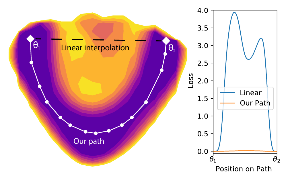
This figure is a two-dimensional slice of a loss function with millions of dimensions. The straight line runs into a large high-loss region in the middle, peaking near 4; the path AutoNEB finds goes around it, with almost no rise in loss along the way.
How low are the saddles?
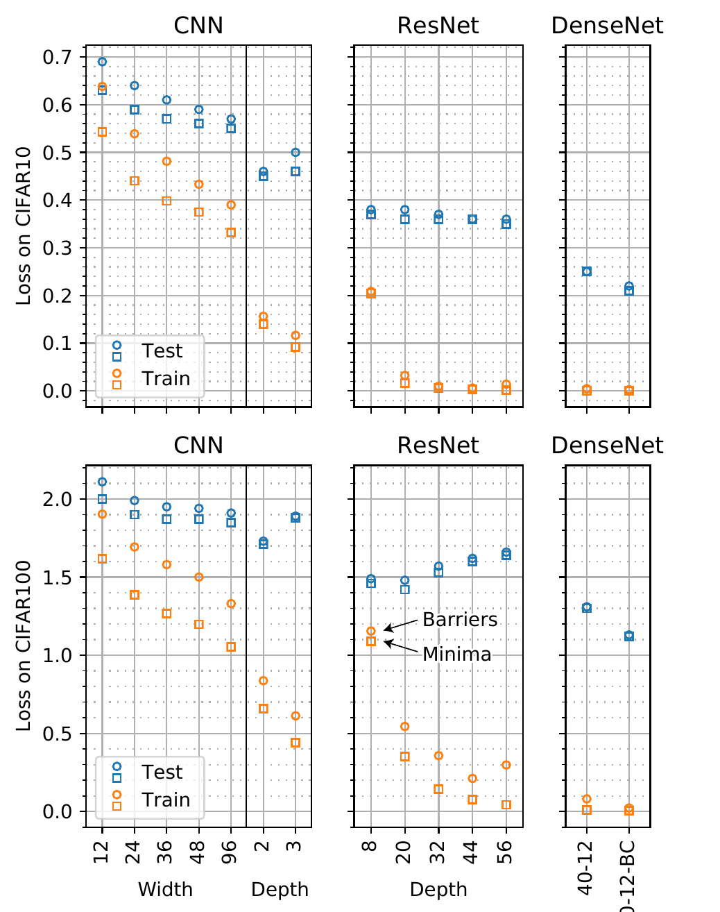
This is the central result of the paper. Read it by comparing squares and dots of the same color. The squares are the average loss at the minima, the dots are the average loss at the saddles on the paths, and the closer the two are, the lower the barrier.
The basic CNNs on the left show the trend. As width grows from 12 to 96, the training-set saddles move steadily closer to the minima, and going deeper to two and three layers closes the gap faster. By the time we reach ResNet and DenseNet, the training saddles on CIFAR-10 sit almost on top of the minima.
Appendix Table B.1 gives the numbers. For ResNet-56 on CIFAR-10, for example, the average training loss is 0.0022 at the minima and 0.0141 at the saddles; for DenseNet-100-12-BC the figures are 0.0005 and 0.0026. In ratio terms they differ several-fold, but the reference point matters. An untrained network's loss on CIFAR-10 is . The saddles of the deep residual networks are about two orders of magnitude below that, and also about an order of magnitude below the same model's loss on the test set.
CIFAR-100 is harder, and its barriers are higher. ResNet-56's training loss rises from 0.0428 to 0.2978, and DenseNet-100-12-BC's from 0.0050 to 0.0223. Compared with the loss of about 4.6 for a randomly initialized network, the gap is still small.
Classification error barely changes either. According to the appendix, the highest error rate along the path exceeds that at the minima by at most 0.7 (CIFAR-10) and 2.9 percentage points (CIFAR-100) for ResNet, and by 0.4 and 1.5 percentage points for DenseNet.
Another yardstick is the point on the training curve where the loss first drops below the saddle. That happens very late. Every architecture has to wait until after the first learning-rate decay, and most ResNets and DenseNets until after the second decay, which is the final stage of training. In other words, these saddles are about as good as “a model that has nearly finished training.”
What the paths look like
The paths themselves are well behaved too. Tracking how individual parameters deviate from straight-line interpolation along a path shows every coordinate moving smoothly, with the largest deviations concentrated near the saddle. The whole path is between 50% and 2.5 times longer than the straight line between its two endpoints.
In their conclusion, the authors suggest these paths might serve as one huge model ensemble, since the test loss along the path is even slightly lower. Garipov et al.'s FGE later developed this direction more fully.
Why so flat?
The paper offers no proof. The authors give two qualitative explanations.
The first is resilience. Modern networks have tens to hundreds of channels per layer, plus skip connections. When one parameter is perturbed slightly, a large number of other parameters can adjust together to compensate, so the model can change its structure step by step without a noticeable rise in loss. Dropout and ensembling exploit and reinforce exactly this resilience, and it is also why a network can be heavily compressed without a noticeable rise in loss.
The second is redundancy, which the authors illustrate with XOR.
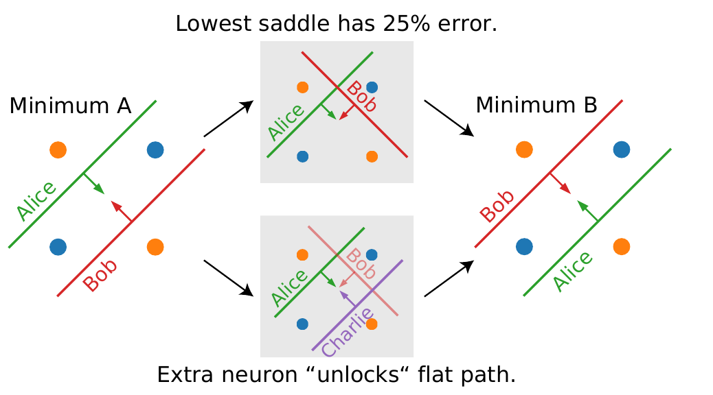
The textbook two-layer perceptron for XOR has two neurons in its hidden layer, which the authors call Alice and Bob. Swapping the two (and swapping the next layer's weights to match) gives another, equivalent minimum. With only two neurons, any continuous path from A to B misclassifies at least one point somewhere along the way; the lowest saddle has a 25% error rate.
Add one more neuron, Charlie, and a relay becomes possible. Charlie first stands in for Bob, Bob gradually moves into Alice's position, Alice then takes over Charlie's job, and finally Charlie leaves. As long as the next layer temporarily ignores whichever neuron is on the move, nothing is misclassified at any point.
The example ties neuron swapping (permutation symmetry) to extra capacity. The question Entezari et al. and Git Re-Basin later kept pursuing is exactly what role permutation symmetry plays in barriers.
Limitations
AutoNEB finds only an upper bound, and the authors acknowledge that they cannot yet characterize when this phenomenon holds. The experiments cover only image classification on CIFAR-10/100, with models no larger than DenseNet-100. Each path costs close to a full training run, so each architecture gets only 10 minima.
Another easy point of confusion is which kind of “connectivity” is meant. This paper shows that a curved low-loss path exists; straight-line interpolation still runs into a high peak. Weight averaging needs the straight line itself to be free of barriers, which is a stricter condition. Later research on linear mode connectivity and permutation alignment deals with exactly that gap.
Conclusion
This paper brought a chemistry tool for finding reaction paths into deep learning and came away with a clean observation for ResNets and DenseNets. Between two independently trained minima there is a path that requires almost no climbing, and the wider and deeper the network, the flatter that path.
So the valley-floor picture needs revising. The low-loss region looks more like one large connected lowland, with the individual minima simply at different spots on it.
The PyTorch implementation is at fdraxler/PyTorch-AutoNEB. Before you actually run it on a large model, work out the budget first. Connecting each pair of minima takes about as long as training the network all over again.