Original paper
Deep reinforcement learning from human preferences
- Publication
- NeurIPS 2017Conference
- First submitted to arXiv
- arXiv:1706.03741
Cite this paper · BibTeX
The citation identifies the linked source version. It cites the original paper and its authors.
@misc{reinforcementlearningrlhumanpreferences2017,
  title = {{Deep reinforcement learning from human preferences}},
  author = {Paul Christiano and Jan Leike and Tom B. Brown and Miljan Martic and Shane Legg and Dario Amodei},
  year = {2017},
  eprint = {1706.03741},
  archivePrefix = {arXiv},
  url = {https://arxiv.org/abs/1706.03741}
}
Say you want Hopper, the one-legged robot in the simulator, to do a backflip. How do you write the reward function?
OpenAI's June 2017 blog post includes one answer, which the authors say took them two hours to write:
def reward_fn(a, ob):
    backroll = -ob[7]
    height = ob[0]
    vel_act = a[0] * ob[8] + a[1] * ob[9] + a[2] * ob[10]
    backslide = -ob[5]
    return backroll * (1.0 + .3 * height + .1 * vel_act + .05 * backslide)
The robot does make it over, but the authors' own verdict is that it's “a lot less elegant.” The same post shows another Hopper that lands steadily after each flip and goes straight into the next one. Whoever trained it wrote no reward function at all. They just watched pairs of clips, one or two seconds each, over and over, and clicked whichever looked more like a backflip. About 900 clicks in total, in under an hour.
The paper is a collaboration between Christiano and Amodei at OpenAI and Leike, Legg and others at DeepMind. The author list also includes one Tom Brown (yes, the same Tom Brown who was first author on the GPT-3 paper three years later). The RLHF (reinforcement learning from human feedback) approach that InstructGPT later cites starts here. There are no language models in this paper, though, only MuJoCo robots and Atari games.
Defining the problem
Deep RL's successes on Atari and Go all rest on the premise that the reward can be written down. Games have scores; Go has wins and losses. But goals like “wipe the table clean” or “scramble some eggs” are hard to write as a function of sensor readings. Write a rough approximation anyway, and the agent often learns to drive that approximate value up without doing what people actually wanted.
There are two existing routes. If you have demonstrations, you can use inverse RL to infer the reward from them, or simply imitate them. But there are many behaviors humans can't demonstrate, such as controlling a robot with lots of joints and a body nothing like a human's. The backflipping Hopper is a case in point. Anyone recognizes a backflip at a glance, but nobody can steer the robot through one by hand.
The other route is to have a person serve as the reward function directly, watching the agent and scoring its behavior in real time. The problem is volume. Deep RL routinely needs hundreds to thousands of hours of experience, and no human can sit there scoring all of it. The authors estimate that the amount of feedback has to come down by several orders of magnitude before this route becomes workable.
The authors set out four goals:
- Solve tasks people can only “recognize” but cannot demonstrate;
- Let non-experts do the teaching;
- Scale to large problems;
- Use feedback sparingly.
Comparisons instead of scores
Instead of asking people for scores, the paper asks them to compare. A trajectory segment is a sequence of observation–action pairs:
A person watches two segments; if they prefer the first, we write .
This setup has a catch. Without a reward, how do you know whether the agent is learning well?
The authors use two kinds of evaluation. The quantitative one assumes human preferences are actually determined by some hidden reward function , so the segment with the higher total reward is the one that gets preferred. That lets the environment's original reward serve as the answer key. The agent never sees it during training, and it's used for scoring once training is over. The qualitative evaluation is for tasks that have no reward function at all, such as the backflip, where all you can do is show the videos to people.
So the main experiments in this paper take tasks that already have a standard reward, deliberately hide that reward, and give the agent only comparison results.
How, then, does “this segment is better than that one” become the per-step reward that reinforcement learning needs?
Solving the problem
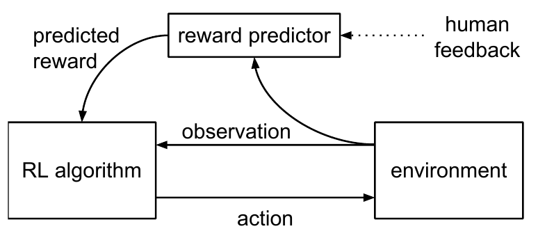
The lower half of the figure is the ordinary RL loop, with the RL algorithm sending actions and the environment returning observations. The difference is where the reward comes from. The environment no longer provides one; instead, the reward predictor at the top scores the observations, and the predictor itself is learned from the human feedback coming in along the dashed line.
The system maintains two neural networks at once, the policy and the reward estimate , updated asynchronously by three processes:
- The policy interacts with the environment to produce trajectories and uses an ordinary RL algorithm to maximize the sum of predicted rewards .
- Pairs of segments are picked from these trajectories and sent to a human for comparison.
- is updated by supervised learning on all the comparisons received so far.
Trajectories flow from 1 to 2, comparisons from 2 to 3, and the parameters of go from 3 back to 1. All three run at the same time, so the human never waits for the agent, and the agent never waits for the human.
Learning a reward from comparisons
The core is step 3. The authors treat as a hidden score that explains human choices, and assume that the probability of a person preferring a segment grows exponentially with the sum of predicted rewards within it:
They then fit the human labels with cross-entropy:
records how the person chose. If they pick the first segment, ; if they pick “equally good,” ; if they pick “incomparable,” the comparison is left out of the database .
This is the Bradley–Terry model from statistics. The authors use chess Elo ratings as an analogy. The rating gap between two players determines who is more likely to win; here, the gap in predicted reward between two segments determines which one the person is more likely to pick.
Let's walk through it with some small numbers. Suppose each segment is 3 steps long and the predictor gives these scores:
import math

r1 = [0.2, 0.5, 0.1]   # r̂ at each step of segment 1
r2 = [0.3, -0.1, 0.0]  # r̂ at each step of segment 2

s1, s2 = sum(r1), sum(r2)            # 0.8, 0.2
p = math.exp(s1) / (math.exp(s1) + math.exp(s2))
print(round(p, 4))                   # 0.6457
The totals differ by 0.6, and the model predicts a 64.6% chance that the person picks segment 1. What gets compared is the total over the whole segment, even though segment 2 actually scores higher on its first step.
If the person does pick segment 1, the loss is ; if they pick segment 2, it's ; pressing “equally good” gives the average of the two, about 0.74. The gradient pushes the two segments' totals toward the person's choice.
The formula also hides two assumptions. First, the sum has no discount factor, which amounts to assuming people don't care whether something happens at the beginning or the end of a segment. Second, only the score difference matters; add a constant to the whole of and the probabilities don't change at all. That's why the authors normalize to zero mean and a fixed standard deviation before handing it to RL.
Keeping the predictor on its feet
On top of the basic version, the authors add three modifications that early experiments found helpful:
- Ensemble: train several predictors (3 in the appendix settings), each on examples drawn from with replacement. Each predictor is normalized separately, and their average serves as .
- Regularization: each predictor holds out of the data as a validation set, and the coefficient is adjusted to keep the validation loss between 1.1 and 1.5 times the training loss; some tasks also add dropout.
- Humans slip: instead of using the softmax above directly, assume there's a 10% chance the person picks at random.
The third one is worth working out. If there's a 10% chance of a random click, the probability of choosing segment 1 becomes , and the 0.6457 from before becomes 0.6311. Not much of a difference. The difference shows up when the score gap is large. With a gap of 10, the original model is almost certain (0.99995) the person will pick segment 1; if they happen to click segment 2, the loss is 10, and the gradient yanks the model hard the other way. With the random-click assumption, the probability tops out at 0.95, and the same wrong label produces a loss of only about 3. One or two misclicks won't drag the whole predictor off course.
Which pair to ask about
Human time is the most expensive resource, so choosing which two segments to show matters. The authors first sample a large number of candidate pairs (10 times the number actually sent, in the appendix settings), have each predictor in the ensemble predict which segment the person will choose, and send the pairs with the most disagreement to the human.
The authors themselves call this a crude approximation. As the ablations later show, on some tasks it actually makes results worse.
The policy side
Once you have , the rest is ordinary reinforcement learning. Atari uses A2C and the robot tasks use TRPO, both policy gradient methods. The authors chose them because keeps changing, which calls for methods that are fairly robust to a changing reward. The hyperparameters mostly follow standard RL settings; the only one tuned is TRPO's entropy bonus. TRPO limits the size of each update with a trust region, and when the reward keeps shifting, it tends not to explore enough.
Closing the loopholes
The appendix has an engineering detail that's easy to miss. The authors found that even without a reward, the environment itself leaks information about the task. In Gym, for example, an episode ends when the robot falls over, so an agent that simply learns “don't let the episode end” has already learned part of the task's goal.
So the authors got rid of every variable-length episode. In the robot tasks, termination conditions were replaced by a penalty that the agent has to learn on its own; in Atari, life-loss and episode-end signals are no longer sent, turning the whole game into one continuous episode.
The score area on the Atari screen is blacked out too, along with the enemy-ship count in BeamRider and the speedometer in Enduro. The robot tasks originally penalized excessive torque, but people can't see torque in a video, so the authors removed that term as well.
The pace of labeling is planned as well. At the start of training, segments from a randomly initialized policy go to people for comparison (500 pairs for Atari). After that the labeling rate decreases over time; for the robot tasks it is roughly proportional to , where is the number of timesteps elapsed. Atari also pretrains the predictor for 200 epochs before starting RL, and during training keeps only the most recent 3,000 labels, looping over them, so that new labels carry enough weight.
Discussion
Robots: 700 labels
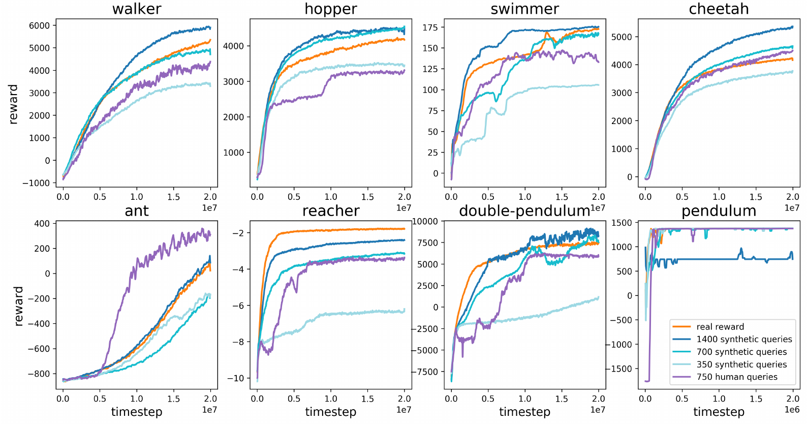
This figure covers 8 MuJoCo tasks. The vertical axis is the true reward, the one the agent never sees during training. The orange line trains directly on the true reward; the three blue lines use 350, 700 and 1400 synthetic labels; the purple line is human labels, 750 according to the legend.
The synthetic labels come from an “oracle” that answers which segment is better according to the segments' total true reward, a labeler who never makes a mistake. The blue lines average 5 runs; the purple line is a single run.
With just 700 labels, the method catches up with RL on almost every task, though the learned reward makes training less stable and more variable. At 1400 labels, tasks such as walker and cheetah even come out slightly above the orange line. The authors' guess is that the learned reward is better shaped, giving positive scores to behaviors that are usually followed by high reward.
Human labels are generally a little worse than synthetic ones, anywhere from half as efficient to just as efficient. Ant is the exception, with the purple line far above the others. The authors asked labelers to prefer segments where “the robot is standing upright,” and that hint turned out to be good reward shaping. The original reward function also has a bonus for staying upright, but it worked less well than human judgment.
Two things to keep in mind when reading this figure. The purple line is a single run, and on Reacher and Cheetah time ran short, so the authors labeled those themselves; the labelers on the other tasks knew neither the environments nor the algorithm. The labeler instructions in the appendix are refreshingly informal, covering everything from how to tell good from bad on each task to asking labelers to ping @tom on Slack when the server has no clips for them. The authors attribute the irregular progress of Hopper's purple line to one labeler not following the planned labeling schedule.
Atari with the score blacked out
The seven Atari games are harder. The legend lists 3.3k, 5.6k and 10k synthetic labels, compared against 5.5k human labels; each synthetic-label curve averages 3 runs.
BeamRider and Pong get close to RL with 3,300 synthetic labels. Seaquest and Qbert get close eventually too, but learn more slowly. SpaceInvaders and Breakout never catch up with RL, though the agent often clears the first level of SpaceInvaders and scores 20 in Breakout, or 50 with enough labels.
On most games, human labels work about as well as synthetic labels with 40% fewer labels. The authors speculate that this may come from labeling mistakes, inconsistency between different labelers on the same training run, or an uneven labeling pace that concentrates labels in a small part of the state space. With human labels, Qbert can't even get past the first level; the authors think Qbert's short clips are hard to make sense of.
Enduro is the opposite. A3C has a hard time learning to pass other cars through random exploration, and the synthetic labels fail along with it. Humans, though, reward any progress toward passing, which amounts to doing reward shaping for the agent. The result beats A3C and is comparable to DQN.
Tasks with no reward function
What this method is ultimately for is tasks whose reward function can't be written. Keeping the same parameters as before, the authors demonstrate three behaviors:
- Hopper doing a series of backflips, landing upright each time: 900 queries, under an hour.
- Half-Cheetah running forward on one leg: 800 queries, under an hour.
- Keeping even with other cars in Enduro: about 1,300 queries and 4 million frames of interaction. The agent stays alongside other cars most of the time but gets confused easily when the background changes.
The authors labeled all three behaviors themselves.
Ablations: which design choices matter
The authors remove parts of the method and watch how the results change. There are six variants: picking queries at random (random queries), using a single predictor (no ensemble), collecting labels only early in training (no online queries), dropping regularization (no regularization), using single frames for the robot tasks (no segments), and having the oracle give the segment's true total reward directly, fitted with mean-squared-error regression (target).
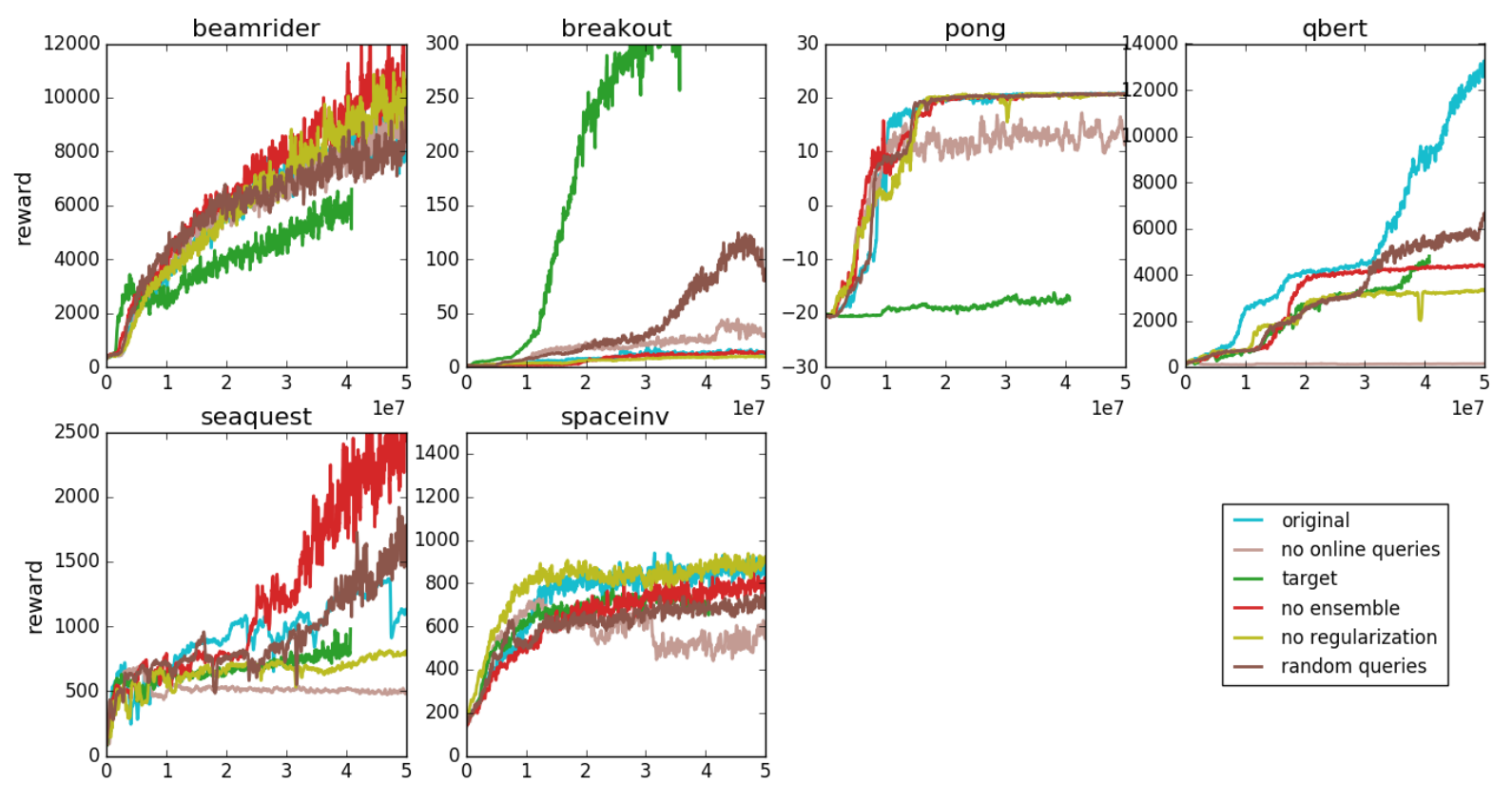
This is the Atari ablation; each line averages 3 runs with 5,500 synthetic labels. The one to watch is no online queries, in light pinkish brown. Pong stalls between 10 and 15 points while the full method (light blue) reaches 20; Qbert is almost zero; Seaquest gets stuck around 500; SpaceInvaders even drops partway through.
The authors' explanation is that labels collected early in training only cover states the early policy visits. Once the policy changes, the agent wanders into places the predictor has never seen. The predictor captures only part of the true reward, and the agent goes off and maximizes that part. Pong makes this concrete. The agent trained offline learns not to lose points but never learns to score, so it keeps volleying back and forth with the opponent, repeating the same exchange forever. Human feedback has to be updated along with the policy; labeling a batch in advance isn't enough.
The results for target are more mixed. On Atari it wins some and loses some. Breakout shoots up to 300 points, far ahead of every other setting, while Pong stalls around -17. The reason is that Atari rewards are clipped to , so the regression mostly just has to predict the sign. Reward scales in the robot tasks vary widely, which makes direct regression hard going; in the MuJoCo ablation, target reaches only about 1,700 on walker against about 4,900 for the full method, and about 1,200 against 4,600 on cheetah. With comparisons, the predictor only has to get the order right, which makes the problem much smoother.
The same goes for single frames. Shrink the MuJoCo segments to 1 step, and walker drops to about 550 and cheetah to about 1,200. The authors found that the longer the segment, the more useful each comparison, but the less efficient it is per frame. When segments are too short, people first have to spend time figuring out what's on screen; only past a certain length does evaluation time grow roughly in proportion to length. The authors chose the shortest length at which evaluation time becomes linear, 1.5 seconds for the robot tasks and 25 timesteps (about 1.7 seconds) for Atari.
The ensemble and active query selection, on the other hand, show no consistent direction. On Qbert the full method is clearly best; on Seaquest, the single-predictor and random-query versions actually come out on top.
Human hours and machine dollars
A footnote in the paper estimates the costs. The Atari experiments ran on a cloud machine with a 16-core CPU and a K80, about 700 US dollars a month; training takes about a day, roughly 25 dollars of compute. 5,000 labels take about 5 hours of human work, about 36 dollars at the US minimum wage. The two are already on the same order of magnitude, so the authors conclude that pushing the number of labels lower would do little for the total cost. (That holds for robots and Atari. Once the setting moved to language models, labeling became the most expensive part; five years later, the labeling team for InstructGPT alone was about 40 people.)
Compared with having a person serve as the reward function directly, learning a separate reward model cuts the amount of interaction that needs a human by about three orders of magnitude.
Agents that fool the judges
The blog post also records a failure case the paper leaves out. A robot arm that was supposed to learn to grasp objects ended up learning to park its hand between the camera and the object. On screen it looked like a grasp, but it never touched anything. The labelers could only judge from what was on screen, so the agent learned to play to the camera. The authors' fix was to add thick white lines to the view to help labelers judge depth.
What the predictor learns is “looks good to a person,” and that's also what the agent maximizes. Wherever people can't tell the difference, the agent has room to game the system. The standing-upright hint made Ant better; the grasping arm is the counterexample. The labelers' eyesight directly determined the quality of the reward.
OpenAI later moved the same pipeline over to language models, trying stylistic continuation and summarization in 2019, large-scale summarization in 2020, and building InstructGPT in 2022. Video clips became pairs of model responses, A2C and TRPO became PPO, and the Bradley–Terry loss barely changed. The problem of pleasing the judges moved over too. The 2020 summarization work found that optimizing too far against the learned reward model actually lowers human-rated summary quality.
Conclusion
People can't write a reward function for a backflip, but they can tell at a glance which clip looks more like one. This paper turns “can tell by looking” into a training signal. On MuJoCo, 700 labels were enough to catch up with the true reward, and the backflip took an hour to teach.
If you want to try this on your own task, the ablations have already sorted out the priorities for you. Always collect labels during training, ask people to compare two segments rather than score them, and make segments long enough for people to see what's going on. Picking queries by ensemble disagreement helps some of the time and hurts some of the time, so it can wait.
That robot arm parking its hand in front of the camera and pretending to grab things was probably the first model to learn to please the judges. Sadly, it wasn't the last.