Original paper
Proximal Policy Optimization Algorithms
- Publication
- Publication venue not yet verified
- First submitted to arXiv
- arXiv:1707.06347
Cite this paper · BibTeX
The citation identifies the linked source version. It cites the original paper and its authors.
@misc{reinforcementlearningppo2017,
  title = {{Proximal Policy Optimization Algorithms}},
  author = {John Schulman and Filip Wolski and Prafulla Dhariwal and Alec Radford and Oleg Klimov},
  year = {2017},
  eprint = {1707.06347},
  archivePrefix = {arXiv},
  url = {https://arxiv.org/abs/1707.06347}
}
If you wanted to train a policy with deep reinforcement learning in 2017, you had roughly three choices, each with its own problems.
DQN is strong on Atari but struggles with continuous control (how much force a robot joint should exert, for example). Vanilla policy gradient methods are simple to implement but waste a lot of data, since each batch of interaction data can be used for only one update. TRPO is more data-efficient and more stable, but it has to solve a constrained optimization problem, approximating second-order information with the conjugate gradient method, and the code gets complicated; TRPO also has trouble when the network uses dropout or when the policy and value function share parameters.
Schulman at OpenAI is TRPO's first author. PPO (Proximal Policy Optimization) is the simplified version he and his colleagues came up with. The goal is to keep TRPO's data efficiency and stability while using only first-order optimization, meaning plain SGD or Adam. In the conclusion, the authors say that turning a vanilla policy gradient implementation into PPO takes only a few lines of code. (In practice there's a lot more to change; more on that later)
InstructGPT later used PPO to fine-tune language models, and PPO became the most common reinforcement learning algorithm in RLHF.
Defining the problem
The most common policy gradient estimator looks like this:
is an average over a batch of samples. When implementing it with automatic differentiation, you write an objective whose gradient is exactly the expression above:
Collecting data is expensive, so it's natural to want to run several optimization steps on the same batch of trajectories. The authors say this isn't well justified, and in experiments it often leads to destructively large updates. The policy jumps too far in one go and performance collapses, and because all the data collected afterward comes from this bad policy, it's hard to recover.
TRPO handles this by adding a constraint to the update:
The KL divergence between the old and new policies can't exceed . That's the “trust region”: look for a better policy only in the neighborhood of the old one.
Theory actually favors replacing the constraint with a penalty, that is, maximizing the objective minus . TRPO doesn't do this because it's hard to pick a that works well across different problems; even within one problem, the right changes from one stage of training to another. The authors also tried a fixed with SGD, and it wasn't good enough.
So can we, with first-order methods alone, safely run several epochs on the same batch of data without letting the policy jump too far?
Solving the problem
Probability ratios and clipping
First, define the probability ratio between the new and old policies:
At the start of an update , so . The objective TRPO maximizes can be written , where CPI stands for conservative policy iteration. Without a constraint, maximizing it pushes very far.
PPO's main objective is the following:
is a hyperparameter, with a default of 0.2 in the paper. The first term inside the min is just ; the second clips the probability ratio to ; and the smaller of the two is taken.
Why take the min? Let's actually work through some numbers. Suppose the old policy gave each sampled action a probability of 0.30, the update moves them to different values, and each comes with a positive or negative advantage:
import torch

eps = 0.2
logp_old = torch.log(torch.tensor([0.30, 0.30, 0.30, 0.30, 0.30]))
p_new = torch.tensor([0.33, 0.39, 0.18, 0.45, 0.18], requires_grad=True)
adv = torch.tensor([2.0, 2.0, -1.0, -1.0, 2.0])

ratio = torch.exp(torch.log(p_new) - logp_old)
unclipped = ratio * adv
clipped = torch.clamp(ratio, 1 - eps, 1 + eps) * adv
objective = torch.min(unclipped, clipped)
objective.sum().backward()

print(ratio.detach())      # tensor([1.1000, 1.3000, 0.6000, 1.5000, 0.6000])
print(objective.detach())  # tensor([ 2.2000,  2.4000, -0.8000, -1.5000,  1.2000])
print(p_new.grad)          # tensor([ 6.6667,  0.0000,  0.0000, -3.3333,  6.6667])
Implementations usually store log probabilities, so the ratio is written as the exponential of their difference. Let's go through the five samples one by one:
- Good action, slightly more likely (, ): still within range, the two terms are equal, and the gradient behaves normally, continuing to push the probability up.
- Good action, already increased too much (): the clipped term is , smaller than the unclipped 2.6, so the min picks the clipped term. The clipped term has zero gradient with respect to the parameters, so this sample no longer drives the update.
- Bad action, already pushed down enough (, ): the clipped term is smaller than the unclipped , so again the clipped term is chosen and the gradient goes to zero.
- Bad action whose probability went up instead (): the unclipped term is smaller, the min picks it, and the gradient is negative, pulling the probability back down.
- Good action whose probability went down instead (, ): the unclipped term 1.2 is smaller than the clipped 1.6, the min picks it, and the gradient still pushes the probability up.
Samples 2 and 3 show what clipping does. A sample that has already gone too far in the right direction can't provide any more reward. Samples 4 and 5 show what the min does. Samples that moved in the wrong direction get no protection from clipping and are penalized as usual. As the authors put it, a change in the probability ratio is ignored only when it would make the objective better, and always counted when it makes the objective worse. That makes a pessimistic lower bound on the unclipped objective.
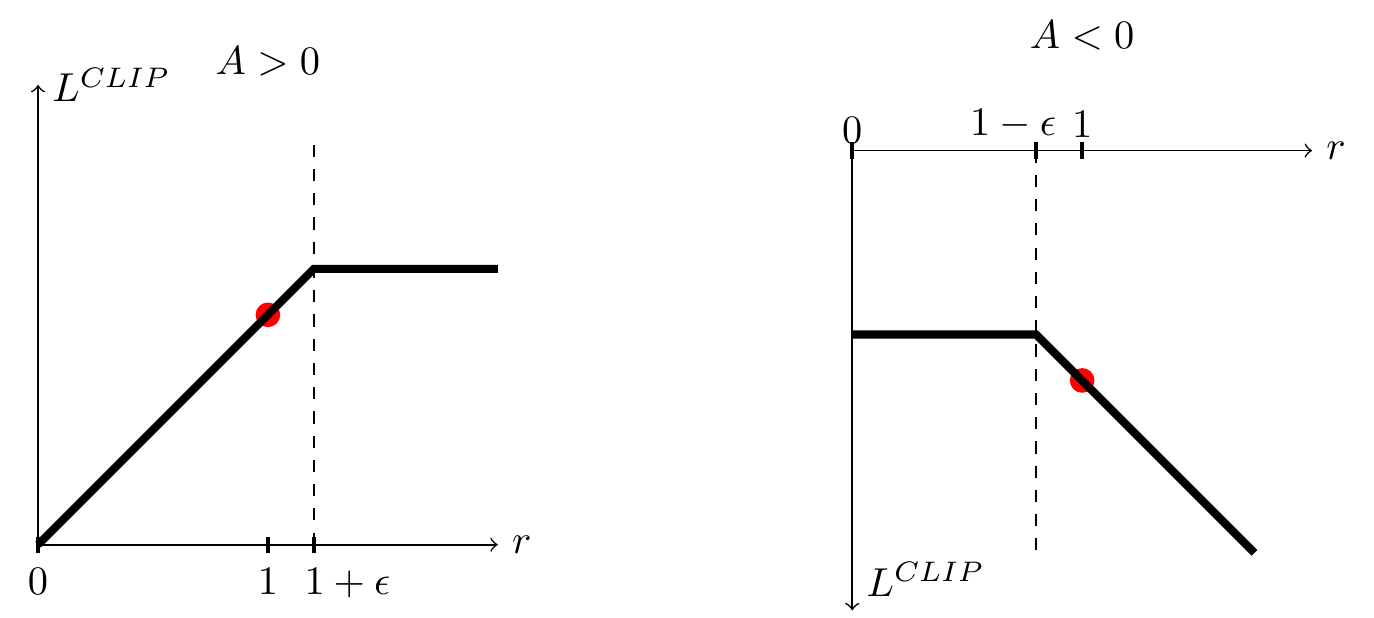
This figure turns the five samples above into curves. On the left the advantage is positive. Starting from the red dot at , the objective rises linearly as you move right, goes flat past , and gives nothing more however far right you go; moving left (the probability drops), it keeps falling with no protection at all. On the right the advantage is negative, everything is mirrored, and the curve goes flat below .
Near , and agree to first order, so the gradient of the first step is the same as without clipping. The two only part ways once the parameters move away from .
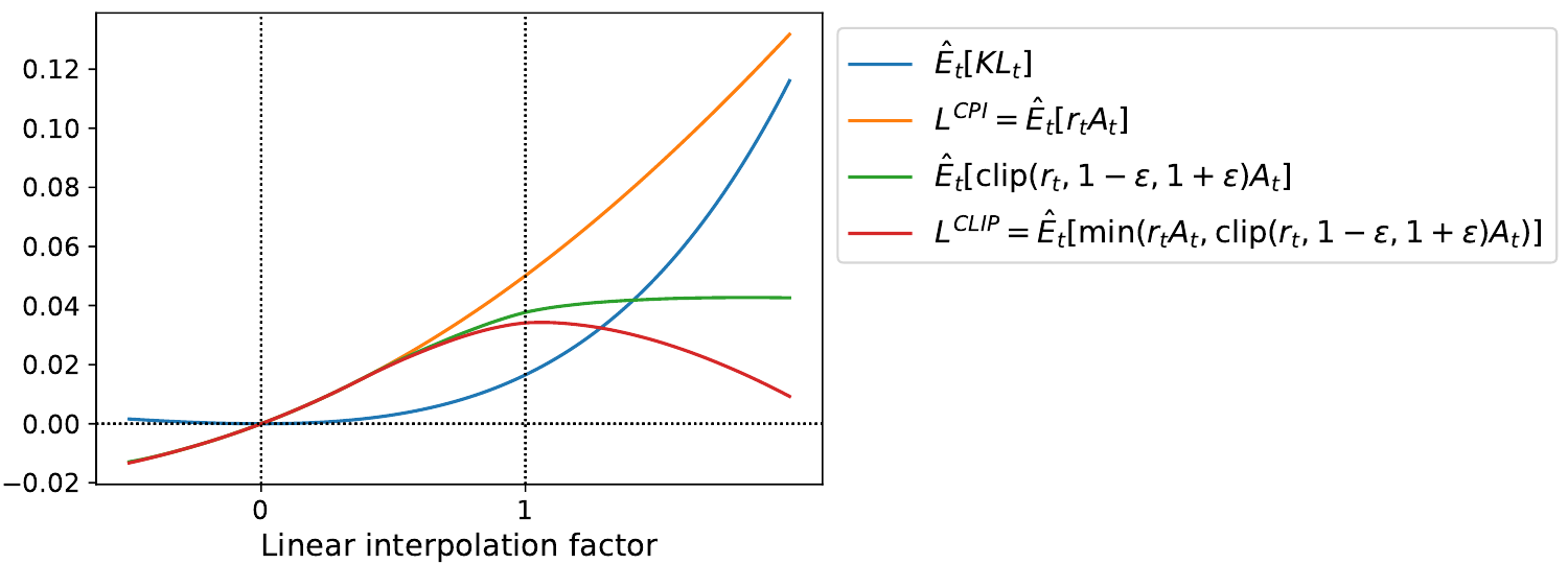
This figure looks at the same thing from another angle. The authors run the first PPO update on Hopper-v1, then interpolate the parameters from the old values (0 on the horizontal axis) along the update direction to the new values (1), and keep going beyond. The orange keeps climbing, as if the farther you go the better; the blue KL keeps rising too. The red , on the other hand, peaks near 1, where the KL is about 0.02, and then falls. The clipped objective has its own “stop here” peak built in, with no extra constraint needed.
Another option: an adaptive KL penalty
The authors also propose an alternative, which serves as an important baseline. The objective is the probability ratio times the advantage minus . After each update, measure the actual mean KL and adjust :
- : . The penalty is too heavy, so ease off a little.
- : . The policy went too far, so penalize harder.
The 1.5 and 2 are heuristic choices. The authors say the algorithm isn't very sensitive to them, and the initial value of gets corrected quickly. Occasionally an update ends up with a KL far from the target, but that's rare.
The full algorithm
In actual training, the policy network often shares parameters with the value network, so the objective combines the policy term, the value function error and an entropy bonus:
is the squared error of the value function, and is the entropy, which encourages exploration.
Advantages are estimated with a truncated version of GAE (generalized advantage estimation):
is the one-step temporal-difference error, and controls how far ahead to look; with it reduces to the finite-horizon estimator used by A3C. The here is the environment reward; don't confuse it with the probability ratio from earlier. The paper uses for both.
The whole procedure is Algorithm 1:
- parallel actors each run the current policy for steps and compute the advantage at every step.
- Using these samples, optimize the objective above for epochs with minibatches of size .
- , then go back to step 1.
Let's plug in the paper's MuJoCo settings. Each iteration collects steps, with minibatches of 64 and 10 epochs, which comes to gradient updates per batch of data. A vanilla policy gradient method does just 1 on the same batch. The Atari setting is 8 actors running 128 steps each, 1,024 steps in total, with minibatches of 256 and 3 epochs, or 12 updates per batch; the clipping parameter is , decayed linearly to 0 over the course of training.
(Funnily enough, when InstructGPT later used PPO to fine-tune language models, it ran only one epoch per batch, so PPO's proudest trick, “reuse the same batch several times,” went unused.)
Discussion
Which surrogate objective works best
The first set of experiments compares different surrogate objectives, sweeping hyperparameters for each. The test environments are 7 MuJoCo continuous control tasks, each trained for 1 million steps with 3 random seeds. The score is the mean total reward over the last 100 episodes, normalized per environment so that a random policy scores 0 and the best result scores 1, and the 21 runs are then averaged into a single number. The policy is an MLP with two layers of 64 units, with no parameter sharing and no entropy bonus.
| Setting | Mean normalized score |
|---|---|
| No clipping, no penalty | -0.39 |
| Clipping, | 0.76 |
| Clipping, | 0.82 |
| Clipping, | 0.70 |
| Adaptive KL, | 0.68 / 0.74 / 0.71 |
| Fixed KL, | 0.62 / 0.71 / 0.72 / 0.69 |
Compiled from Table 1 of the paper.
The version with no clipping and no penalty scores below zero, mainly because its HalfCheetah score is worse than a random policy's, exactly the destructively large updates described earlier. Among the clipped versions, is best; the best settings of the two KL penalties land between 0.72 and 0.74, close to each other but both below clipping. The authors also tried clipping in log space, and it was no better.
Against other algorithms
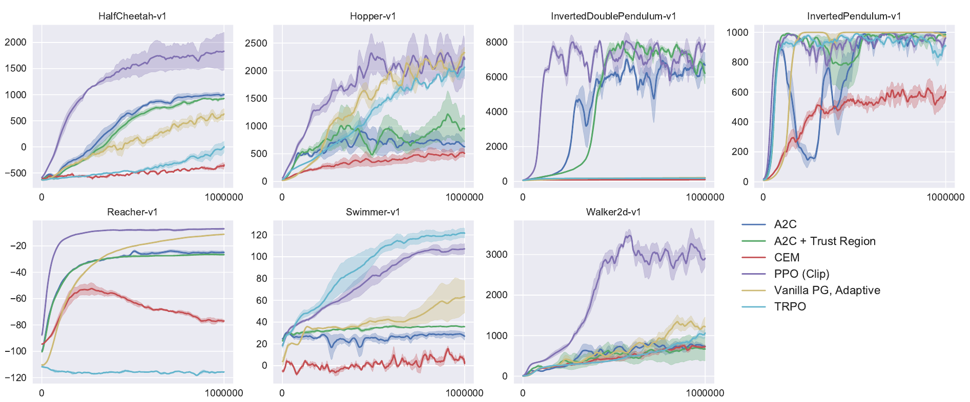
The purple line is PPO. The comparisons include a tuned TRPO, the cross-entropy method (CEM), vanilla policy gradient with an adaptive step size, A2C, and A2C with a trust region. The authors conclude that PPO wins in almost every environment. The biggest gap is on Walker2d, where PPO reaches around 3,000 and every other method stays below 1,200; PPO also leads clearly on HalfCheetah. Swimmer is the exception, with TRPO (the light blue line) ending slightly above PPO.
The authors also show PPO on Roboschool's 3D humanoid robots, with tasks including running forward, chasing a randomly moving target, and getting up off the ground while being pelted with cubes. This set of experiments has only learning curves and footage, with no comparison against other algorithms.
Atari: fast learner, mixed final scores
On Atari the comparison is against A2C and ACER. All three use the same network architecture, and the hyperparameters for A2C and ACER were tuned for this benchmark. Across 49 games with 3 runs each, the number of games each algorithm wins is counted under two metrics:
| Metric | A2C | ACER | PPO | Tie |
|---|---|---|---|---|
| Average episode reward over all of training | 1 | 18 | 30 | 0 |
| Average reward over the last 100 episodes | 1 | 28 | 19 | 1 |
Compiled from Table 2 of the paper.
The first metric favors methods that learn fast; the second favors final performance. PPO leads clearly on the former, while ACER wins more games on final performance. The per-game scores in the appendix have extreme cases on both sides. On Enduro, A2C and ACER both score 0 while PPO gets 758; on Kangaroo it's 45 and 50 against 9,929. Going the other way, ACER scores 37,802 on Gopher against PPO's 2,933, and on DemonAttack it's 38,808 against 11,378. The authors' verdict on ACER is that it performs similarly, but PPO is much simpler.
Is clipping actually doing the work?
PPO quickly became the default algorithm, and later research started asking where its performance really comes from.
In Implementation Matters in Deep Policy Gradients (2020), Engstrom and colleagues at MIT focused on some “small details” in the official implementation, such as clipping the value function loss too, scaling rewards by the standard deviation of the discounted return, orthogonal initialization, Adam learning rate annealing, observation normalization and clipping, and clipping the global gradient norm to 0.5. The PPO paper itself doesn't emphasize any of these. Engstrom et al. conclude that most of PPO's advantage in cumulative reward over TRPO comes from these code-level optimizations.
They also measured the probability ratios. During PPO training, the largest ratio keeps exceeding ; clipping doesn't confine the policy to that range. The code from earlier shows why. Clipping only zeroes the gradient of the samples that are out of range, but all samples share the same parameters, so the gradients of the other samples still push the parameters forward and, along the way, push the out-of-range sample even further out. At the start of the first epoch every , so that step is exactly the same as without clipping, and how big it is depends on how steep the objective is.
They also built PPO-NoClip, which keeps these code-level details but removes the clipping. On Walker2d, Hopper and Humanoid it scores 2,867, 2,371 and 831, against 3,292, 2,513 and 806 for standard PPO. Walker2d still shows a gap of about 400 points, the Hopper gap is around the size of the confidence interval, and on Humanoid the unclipped version actually comes out slightly higher. PPO-M, a minimal version that keeps the clipping but drops the code-level details, scores below PPO-NoClip on all three. Their conclusion is that clipping often matters less than these code-level details.
Another frequently cited write-up is The 37 Implementation Details of Proximal Policy Optimization, published by Huang et al. on the ICLR blog track in 2022. They went through the OpenAI baselines implementation line by line and catalogued 13 core details, plus extra details for settings such as Atari, continuous control and LSTMs. For example, advantage normalization happens within each minibatch, not over the whole batch; as for value function clipping, Engstrom et al. found no evidence that it helps, and another large-scale study even suggests it hurts. They also mention that even the original implementation doesn't produce very consistent results.
None of this research overturns PPO, which is still one of the best-performing setups in these experiments. What it corrects is the account of why PPO works. The clipped objective makes multi-epoch updates safer, but to reproduce the paper's numbers reliably, the code details that never made it into the paper matter just as much.
Applying it to language models
With a language model, each token is an action and a whole response is a trajectory. On top of PPO, InstructGPT added a KL penalty against the SFT model to keep the model from drifting too far in its effort to please the reward model. Later, DeepSeek's GRPO dropped the value network and estimates advantages by comparing the scores of several responses to the same question against one another, while keeping the clip-plus-min formulation.
Conclusion
The core of PPO is a one-line objective. The clip stops samples that have gone too far in the right direction from earning more, and the min makes sure samples that went the wrong way still lose points. With that, you can safely run several more epochs on the same batch of data.
If you're going to implement it yourself, the paper's formulas only get you halfway. The paper never mentions details like advantage normalization, reward scaling and value function clipping, yet the results lean heavily on them. The least painful route is to go down that list of 37 details and check them off one by one.
Over the years people have kept stripping parts out of PPO. DPO stripped out the reinforcement learning, GRPO stripped out the value network. That clip, though, is still with us.