Original paper
StrongSORT: Make DeepSORT Great Again
- Publication
- IEEE Transactions on Multimedia 2023Journal
- First submitted to arXiv
- arXiv:2202.13514
Cite this paper · BibTeX
The citation identifies the linked source version. It cites the original paper and its authors.
@misc{multiobjecttrackingstrongsort2022,
  title = {{StrongSORT: Make DeepSORT Great Again}},
  author = {Yunhao Du and Zhicheng Zhao and Yang Song and Yanyun Zhao and Fei Su and Tao Gong and Hongying Meng},
  year = {2022},
  eprint = {2202.13514},
  archivePrefix = {arXiv},
  url = {https://arxiv.org/abs/2202.13514}
}
Multi-object tracking leaderboards were getting harder and harder to read.
Every paper used a different detector: some Faster R-CNN, some CenterNet, some YOLOX. The re-ID models differed too, the amount of extra training data varied, and each method added its own little tricks at inference time. When one method beat another by two points, it was hard to say whether the association algorithm was better, the detector was stronger, or someone had thrown in one more trick.
Yunhao Du and colleagues at Beijing University of Posts and Telecommunications decided to go back and take another look at an old friend, DeepSORT.
This 2017 tracker is simple, easy to extend and widely used in engineering, but it had long since fallen behind on the leaderboards. The authors argue that it fell behind because its parts were outdated, which has nothing to do with the tracking framework itself. So swap in new parts one at a time and see how far it can go.
The paper's title is "Make DeepSORT Great Again."
Read enough papers and you'll notice that these days everyone is very busy making things great again. RepVGG set out to make VGG great again, and the very next year someone wanted to make RepVGG "even greater." GCN, FCN, encoder-decoders, LoRA, even Sigmoid with MSE are all lined up waiting to be great one more time. A perfectly good campaign slogan, and the research community has used it until it's practically moldy. (Dear authors, this joke really can retire now.)
Fortunately, DeepSORT, whose turn it is this time, really does deliver the results.
Defining the problem
The authors want to solve two things.
The first is fair comparison. They want to provide a strong and fair baseline, using today's good detectors and re-ID models plus a curated set of inference tricks. Only by comparing against this baseline can a new method know where its contribution lies. The authors also state explicitly that this part claims no algorithmic novelty; the contribution is taking DeepSORT apart cleanly and fitting it with new parts.
The second is two kinds of "missing" inherent in multi-object tracking:
- Missing association: the same object is cut into several short tracklets. Online trackers lack global information, so this happens to them especially often.
- Missing detection: an object is treated as background, which is to say it's a missed detection, usually caused by occlusion or resolution that's too low.
Existing solutions each come at a cost. To link short tracklets into long tracks, the usual approach is an offline global link model, but most of these rely on appearance features and are computationally heavy. To fill in missed detections, linear interpolation is common, but linear interpolation ignores motion information completely.
Solving the problem
First, take DeepSORT apart
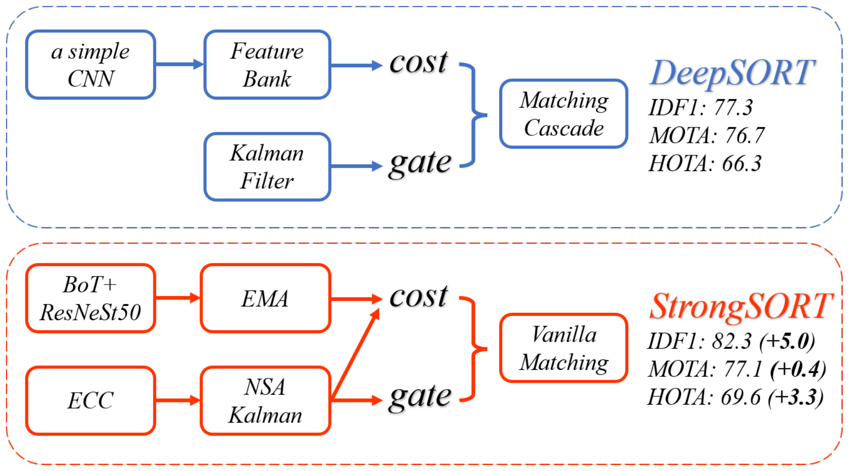
The authors treat DeepSORT as two branches.
Appearance branch: a simple CNN pretrained on the MARS pedestrian dataset extracts features for each detection box. Each track keeps the features from its last 100 frames as a feature bank. The appearance distance between a new detection and a track is the cosine distance between the detection and the most similar feature in the bank.
Motion branch: a Kalman filter predicts where the track will be in this frame, and the Mahalanobis distance is used as a gate to rule out impossible matches.
Finally, the matching cascade splits matching into several subproblems, letting the most recently seen tracks choose first.
For a fair comparison, the detector has to be unified first. The scores in the top half of the figure are the result after the authors switched DeepSORT's detector to the same YOLOX-X that ByteTrack uses. With detection held constant, any remaining gap comes from the tracker itself.
Replacing one part at a time
A stronger appearance model (BoT). The original simple CNN is replaced with BoT, a strong baseline in re-ID that collects many training tricks, with a ResNeSt50 backbone pretrained on DukeMTMC.
EMA feature updates. DeepSORT's feature bank also stores the features of the occasional very poor-quality detection. The authors instead use an exponential moving average to maintain each track's appearance state:
is the feature of the detection matched in this frame, and . The old appearance state accounts for 90% and the new frame for only 10%, so noise in a single frame is less likely to pull the appearance off course. It also means distances no longer have to be computed one by one against the 100 features in the bank, so it's faster.
Camera motion compensation (ECC). MOTChallenge, DanceTrack and KITTI all have videos with camera motion. The authors use enhanced correlation coefficient (ECC) image alignment to estimate the global rotation and translation between two adjacent frames, and first move the tracks' predicted positions along with the camera. This is the same method Tracktor++ uses.
The NSA Kalman filter. An ordinary Kalman filter treats the observation noise of every detection box as the same. The NSA (Noise Scale Adaptive) Kalman filter, borrowed from GIAOTracker, adjusts the observation noise according to the detection score:
is the detection score. For a box scoring 0.9, the observation noise is down to a tenth of the original, so the filter trusts it more; for a box scoring 0.6, 40% of the noise remains, so the filter relies more on its own prediction.
Motion cost. In DeepSORT's experiments, the cost was appearance distance alone, and motion served only as a gate. StrongSORT combines the two into a weighted cost:
This weight follows the setting used by FairMOT and other methods.
Ordinary matching. Finally, the matching cascade is removed and replaced with a single global linear assignment. We'll get to the reason when we look at the ablations.
Two add-ons: AFLink and GSI
The tracker with all these parts installed is called StrongSORT. The authors also propose two lightweight, model-independent post-processing algorithms that don't use appearance features; with these added, it's called StrongSORT++. Both algorithms need to see the tracks of the whole video, so StrongSORT++ is an offline method.
AFLink (Appearance-Free Link): linking broken tracks back together.
AFLink looks only at the spatiotemporal information of two short tracklets to decide whether they belong to the same object. Each tracklet takes its last 30 frames, with three numbers per frame: frame index and position , ; tracklets shorter than 30 frames are zero-padded. So a tracklet is a small matrix.
The two tracklets each go into their own branch, and the two branches don't share weights:
- Temporal module: four Conv-BN-ReLU layers with kernels that convolve only along the time dimension, with 32, 64, 128 and 256 channels in turn.
- Fusion module: one convolution that fuses the information from the three dimensions, frame index, and .
The outputs of the two branches are pooled, flattened and concatenated, then fed into a classifier with two fully connected layers, which outputs the probability that the two tracklets belong to the same object.
The training data is cut straight from ground-truth tracks. Annotated tracks are cut into tracklets with random spatiotemporal noise added, at a 1:3 ratio of positive to negative samples, and trained with binary cross-entropy for 20 epochs. The whole training run takes only a little over ten seconds.
At inference time, track pairs more than 30 frames apart in time or more than 75 pixels apart in space are first ruled out. Then AFLink's score is used as the similarity for a single linear assignment, and a pair is linked only if its score is above 0.95.
GSI (Gaussian-Smoothed Interpolation): filling gaps and smoothing out jitter along the way.
Linear interpolation draws a straight line between the two ends of a gap, regardless of how the object actually moved. GSI treats each track's box position as a function of time and fits it with Gaussian process regression:
is the box's in frame , and is Gaussian noise. Given the frames to predict, the smoothed positions are computed from the Gaussian process's posterior mean:
The kernel width controls how smooth the track is, and the authors adjust it according to the track length : , with . The maximum gap for interpolation is 20 frames.
GSI does more than fill gaps. It refits the whole track, so the small frame-to-frame jitter of the original detection boxes gets smoothed out too. The authors see it as a kind of filter for detection noise: tracks from linear interpolation have very jittery velocity curves, while with GSI they're much steadier, which helps downstream applications that need to estimate velocity.
Discussion
The detector is YOLOX-X, trained the same way as in ByteTrack. At inference time, the NMS threshold is 0.8, the detection score threshold 0.6 and the matching distance threshold 0.45. The ablations split each video in the MOT17 training set into first and second halves, and all experiments run on a single V100.
What each part is worth
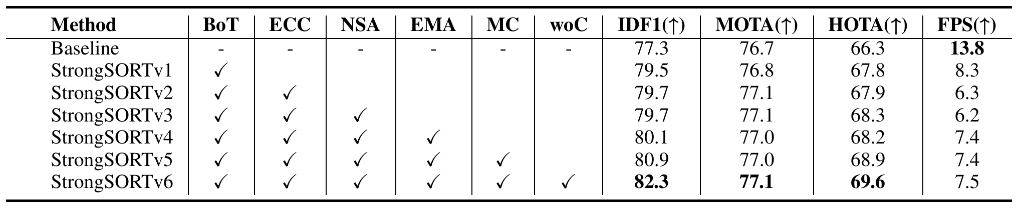
Reading from top to bottom, each row adds one more part:
- BoT: IDF1 +2.2, HOTA +1.5. Better appearance features help more than any other change, but FPS drops from 13.8 to 8.3.
- ECC: IDF1 +0.2, MOTA +0.3, and FPS drops further to 6.3.
- NSA: HOTA +0.4, with MOTA and IDF1 unchanged. What improves is localization accuracy, which is exactly the part HOTA counts and MOTA and IDF1 barely do.
- EMA: IDF1 +0.4, and FPS climbs back to 7.4.
- Motion cost: IDF1 +0.8.
- Removing the matching cascade: IDF1 +1.4, HOTA +0.7.
After all six steps, IDF1 goes from 77.3 to 82.3 and HOTA from 66.3 to 69.6, while MOTA gains only 0.4. What these parts improve is mainly association; detection stays the same.
Speed, meanwhile, drops by almost half.
Why remove the matching cascade
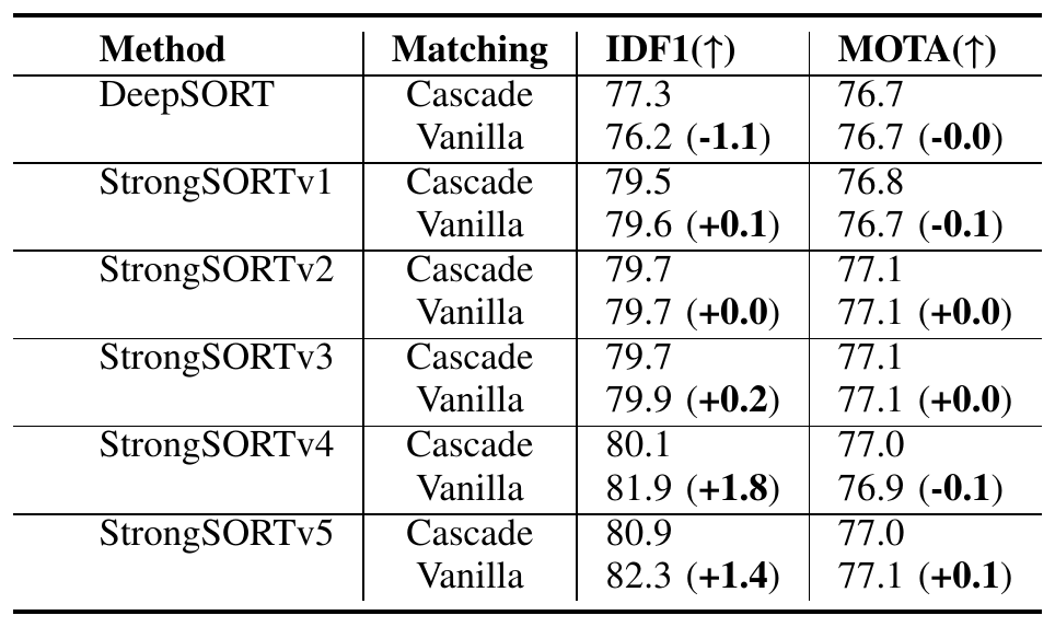
This table compares the cascade and ordinary matching on every version.
For the original DeepSORT, the cascade helps; without it, IDF1 drops 1.1. But the stronger the tracker, the smaller the cascade's benefit. By v4 and v5, removing the cascade actually raises IDF1 by 1.8 and 1.4.
We saw the motivation for the cascade in the DeepSORT note. The Mahalanobis distance favors uncertain tracks, so the most recently seen tracks get to choose first. The authors conclude that this prior reduces confusing matches in a weak tracker, but once appearance features are strong enough and the cost includes motion information too, the tracker rarely mixes people up to begin with, and this extra constraint ends up tying its hands.
What AFLink and GSI can be attached to
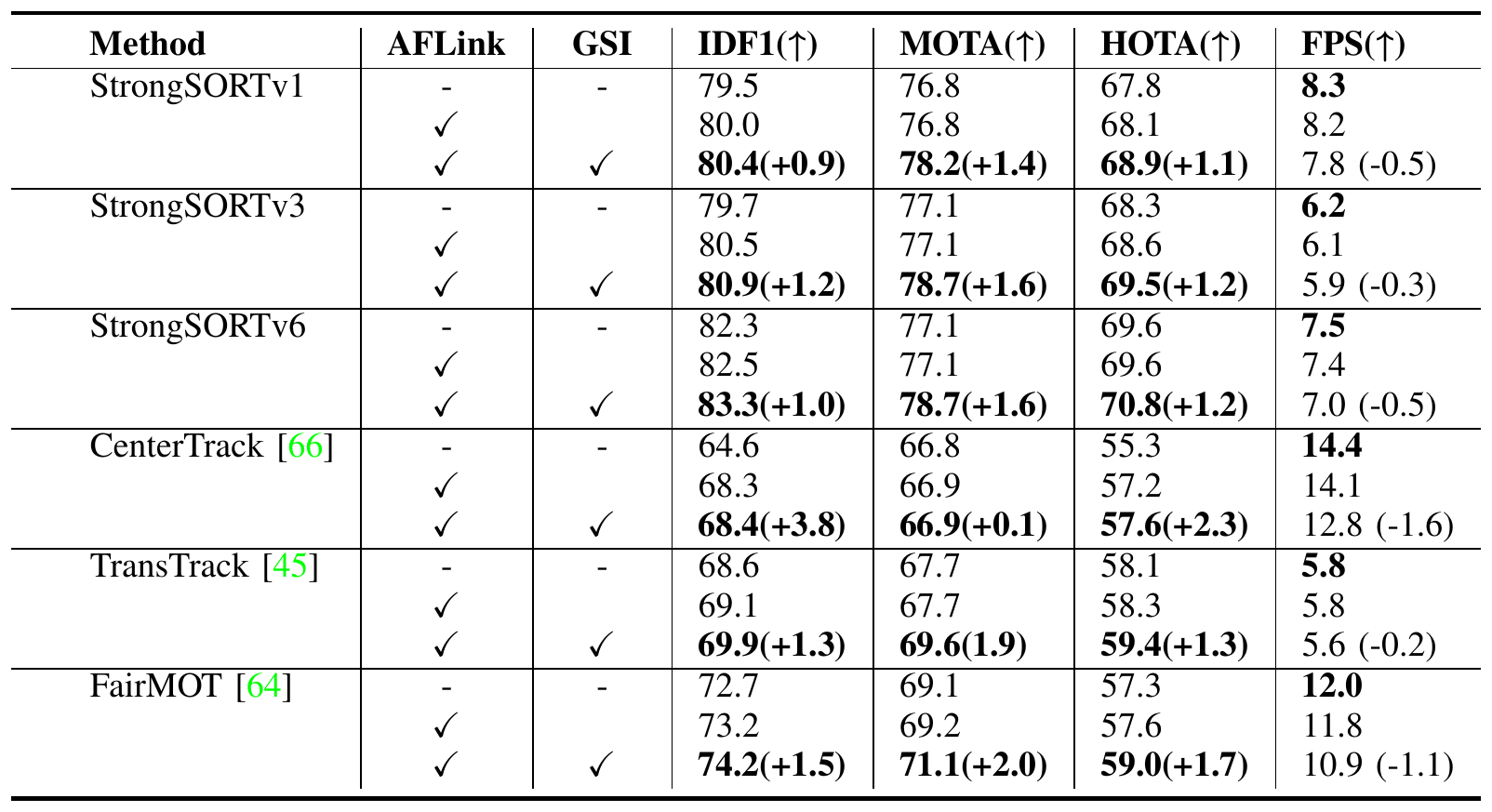
Each tracker has three rows: the original, with AFLink, and with GSI added on top.
AFLink helps weaker trackers more. CenterTrack only does local matching between adjacent frames, so whenever a blocked person's track breaks, it becomes a new track; with AFLink, IDF1 goes up 3.7. StrongSORTv6 breaks tracks less often to begin with and gains only 0.2.
According to the authors, GSI is the opposite: the stronger the tracker, the more useful it is. It improves both MOTA and HOTA, since the filled-in boxes reduce missed detections and the smoothed boxes sit closer to the true positions. But if a track has many wrong associations to begin with, GSI will smooth the wrong track out beautifully too.
On MOT17, the two cost 1.7 ms and 7.1 ms per image, respectively.
Leaderboards
On the MOT17 test set, StrongSORT has HOTA 63.5, IDF1 78.5, MOTA 78.3 and 1446 ID switches. The authors' YOLOX reproduction of DeepSORT gets 61.2, 74.5, 78.0, and their reproduction of ByteTrack (without linear interpolation) gets 62.8, 77.2, 78.9. With the same detector, StrongSORT's association beats both, and its MOTA is about the same as ByteTrack's.
StrongSORT++, with AFLink and GSI added, gets 64.4, 79.5, 79.6. Its HOTA, IDF1, AssA and DetA were all first at the time, and its IDF1 and AssA were both 2.1 ahead of second place.
On MOT20, StrongSORT++ has HOTA 62.6, IDF1 77.0 and only 770 ID switches, but its MOTA of 73.8 is below the 77.8 reported in the ByteTrack paper. The authors explain that they kept MOT17's detection score threshold, which missed a lot of people in the crowded MOT20: StrongSORT++'s FN is 117,920, while ByteTrack's is only 87,594. That's exactly the problem the ByteTrack paper set out to solve.
On DanceTrack, StrongSORT++ has a HOTA of 55.6, slightly higher than OC-SORT's 55.1. Interestingly, on DanceTrack the authors removed BoT and EMA, the two appearance-related improvements. The dancers all dress about the same, so appearance features don't help.
Limitations the authors admit
First, it's slow. The DeepSORT-style framework needs an extra re-ID model, and StrongSORT runs at only 7.5 FPS on MOT17 and 1.5 FPS on MOT20. Second, the detection threshold is too high, so MOTA on MOT17 and MOT20 is on the low side. Third, AFLink can only link broken tracks back together; it can't split apart tracks that have been merged.
Afterward
StrongSORT did become a common baseline, and later methods such as Deep OC-SORT include it in their comparison tables. BoT-SORT, later the same year, took a similar route, adding camera motion compensation and re-ID fusion to ByteTrack. Open-source tracking packages like BoxMOT also added StrongSORT to their lists of interchangeable trackers.
Conclusion
No new tracking framework, just one part after another swapped for a newer one. StrongSORT replaces DeepSORT's detector, appearance model, feature updates, Kalman filter, cost and matching in one round, and shows that a 2017 framework can still rank near the top in 2022. The genuinely new things are AFLink and GSI, two post-processing steps that use no appearance, finish in a few milliseconds and can be attached to the back of any tracker.
It breaks a "strong tracker" down into step-by-step increments. Swapping the re-ID model is worth 2.2 IDF1, removing the matching cascade is worth 1.4, and after the whole set of swaps, speed falls from 13.8 FPS to 7.5 FPS. When you're picking tricks, this price list comes in very handy.
Four months later, BoT-SORT fitted similar camera compensation and re-ID onto ByteTrack and pushed MOT17 a little further forward.