Original paper
Object-Centric Learning with Slot Attention
- Publication
- NeurIPS 2020Conference
- First submitted to arXiv
- arXiv:2006.15055
Cite this paper · BibTeX
The citation identifies the linked source version. It cites the original paper and its authors.
@misc{multiobjecttrackingslotattention2020,
  title = {{Object-Centric Learning with Slot Attention}},
  author = {Francesco Locatello and Dirk Weissenborn and Thomas Unterthiner and Aravindh Mahendran and Georg Heigold and Jakob Uszkoreit and Alexey Dosovitskiy and Thomas Kipf},
  year = {2020},
  eprint = {2006.15055},
  archivePrefix = {arXiv},
  url = {https://arxiv.org/abs/2006.15055}
}
This isn't a tracking paper.
It shows up in this series because someone later used it for multi-object tracking. Before getting there, we need to understand what it does.
In 2020, a team at Google Brain proposed Slot Attention. On the author list, the corresponding author, Thomas Kipf, is the author of GCN, and one of the advisors, Alexey Dosovitskiy, published ViT a few months later. That same year, DETR used a set of object queries to recast detection as set prediction, and TrackFormer and MOTR later turned object queries into track queries. What Slot Attention does is somewhat similar to DETR, but its starting point is completely different. It gives no annotations at all and lets the model break the scene into individual objects by itself.
Defining the problem
The feature maps a convolutional network extracts are a "distributed" representation. Each position on the feature map mixes information about everything near that position; how many objects are in the image, and where each one is, isn't explicitly separated out.
Yet many tasks that require reasoning want their input as a set of objects, such as a red cube here and a green cylinder there. Physical simulation, multi-agent systems and visual reasoning all operate on objects as their units. The authors call this kind of representation object-centric.
The trouble is that getting one from raw images is hard, usually requiring supervision or an architecture designed for a specific task. So many studies simply skip this step and take object states straight from a simulator or game engine.
The existing approaches each have their problems:
- IODINE and MONet, unsupervised scene decomposition models, have to repeat "decode, compare with the original image, encode again" for several rounds, so training is slow.
- In capsule networks, each capsule specializes in a certain kind of object, so they fail to generalize to combinations they haven't seen.
- In set prediction methods such as DETR and Set Transformer, each query has its own set of learnable parameters. Train with 100 queries, and at test time you can only have 100.
The authors want a module that can be attached directly after a convolutional network. It takes feature vectors as input and outputs "slots," each describing one object. Moreover, every slot looks the same, any of them can bind to any object, and their number can change at test time.
Solving the problem
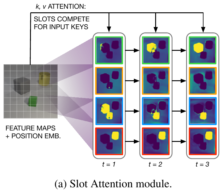
Read this figure from left to right. The feature map on the left is the input, and on the right is where each of the four slots is looking across the three iterations. At first every slot's gaze is blurry, and the further along it goes, the more each slot concentrates on a single object.
One iteration
To begin, slots are sampled at random from the same Gaussian distribution:
and are learnable parameters shared by all slots. That's why the number of slots can change at test time; you just sample as many as you need.
Then repeat times (the paper uses ). Each iteration first uses three linear projections to turn the inputs into keys and values and the slots into queries , and computes the dot-product attention scores:
Ordinary attention takes the softmax for each query along the inputs dimension; Slot Attention reverses this, taking the softmax for each input along the slots dimension:
In other words, each input feature has to divide its total of 1 among the slots.
Next, each slot takes a weighted mean of the inputs assigned to it as its update:
Finally a GRU, with the previous iteration's slots as its state and this iteration's updates as its input, computes the new slots, followed by an optional residual MLP. The inputs and slots both go through LayerNorm at the start of every iteration.
Working through it once
Let's walk through it with 4 inputs and 2 slots. Suppose the computed scores are:
| slot 1 | slot 2 | |
|---|---|---|
| Input 1 | 2.0 | 0.0 |
| Input 2 | 1.5 | 0.5 |
| Input 3 | 0.0 | 1.8 |
| Input 4 | 0.2 | 2.2 |
Take the softmax across each row, and each input divides itself between the two slots:
| slot 1 | slot 2 | |
|---|---|---|
| Input 1 | 0.881 | 0.119 |
| Input 2 | 0.731 | 0.269 |
| Input 3 | 0.142 | 0.858 |
| Input 4 | 0.119 | 0.881 |
Slot 1 mainly gets inputs 1 and 2, and slot 2 mainly gets inputs 3 and 4. Normalizing each column, slot 1's weighted-mean weights are 0.470, 0.390, 0.076 and 0.064, and slot 2's are 0.056, 0.126, 0.403 and 0.414. The two slots act like two cluster centers, each taking its own group of inputs.
Why reverse the softmax? Suppose the two slots happen to be identical, with the same query, so both columns of scores are 2.0, 1.5, 0.0, 0.2.
- With ordinary attention, taking the softmax over the inputs, the two slots get exactly the same weights, 0.524, 0.318, 0.071 and 0.087. Both stare at inputs 1 and 2, and nobody looks after inputs 3 and 4.
- With Slot Attention's approach, each input splits itself evenly between the two slots, 0.5 each. Neither can take anything away from the other, and inputs 3 and 4 are guaranteed to go to someone.
Every input has to be assigned to some slot, so the slots compete; for one slot to take a bit more, the others have to take a bit less. Through the GRU update and into the next iteration, tiny initial differences get amplified, until each slot locks onto its own object. The authors' ablation in the appendix bears this out. Switching the softmax back to run over the inputs clearly hurts performance on both tasks.
And why a weighted mean rather than a weighted sum? Because the scores are normalized over slots, the total each slot receives isn't fixed. In the example above it's 1.873 and 2.127, and a slot that gets no object can approach 0. With a weighted sum, the size of the update would swing up and down along with it; with a mean, training stays stable.
The whole module's computational cost is .
Symmetry
The authors prove that Slot Attention has two properties: it's invariant to the order of the inputs and equivariant to the order of the slots. Shuffle the inputs and the output stays the same; shuffle the order of the initial slots and the output is simply shuffled the same way.
This guarantees that every slot represents objects in the same format; there's no such thing as "slot 1 handles the cubes." DETR's object queries are different. Each query has its own parameters, and after enough training, each one often develops a preference for certain positions or sizes.
Two ways to use it
Unsupervised object discovery. Put Slot Attention inside an autoencoder. The encoder is a convolutional network with position embeddings, followed by Slot Attention; the decoder expands each slot separately into an image, outputting RGB and a mask. The masks of all slots go through a softmax across slots and serve as mixing weights to combine the individual images into one, which is compared against the original image for reconstruction error. The whole process needs no annotations at all.
Supervised set prediction. Same encoder, with each slot fed into a shared MLP that predicts the object's properties. Both the predictions and the labels come in arbitrary order, so they're matched with the Hungarian algorithm, just as in DETR.
Discussion
Object discovery
The authors evaluate on three synthetic datasets: CLEVR6 (CLEVR 3D scenes with at most 6 objects), Multi-dSprites (colored 2D shapes) and Tetrominoes (Tetris pieces). The metric is ARI, which measures how well the segmentation agrees with the real objects, excluding the background; 100 is perfect.
| Method | CLEVR6 | Multi-dSprites | Tetrominoes |
|---|---|---|---|
| Slot Attention | 98.8 | 91.3 | 99.5 |
| IODINE | 98.8 | 76.7 | 99.2 |
| MONet | 96.2 | 90.4 | — |
| Slot MLP | 60.4 | 60.3 | 25.1 |
Compiled from Table 1 of the paper, ARI (%), averaged over five random seeds. Tetrominoes excludes one failed training run.
Slot MLP is a baseline that replaces Slot Attention with an MLP, so its output slots have a fixed order. Its scores are far lower, which shows that the design of "every slot has the same format and can bind to any object" is necessary.
Slot Attention ties or beats IODINE, and the real gap is in efficiency. On CLEVR6, a single 16 GB V100 can handle a batch size of 64, where IODINE manages only 4; training on 8 V100s takes about 24 hours, versus roughly 7 days for IODINE.
The authors also own up to a failure mode. On Tetrominoes, a training run occasionally gets stuck in a solution that cuts the image into horizontal stripes, one run out of five. When that happens the reconstruction error is clearly higher, so it's visible during training; the score in the table excludes that run.
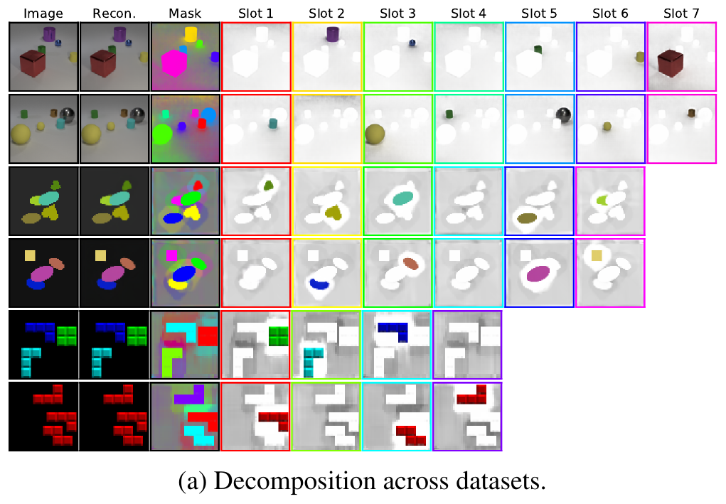
The figure shows that when there are more slots than objects, the extra slots stay blank, getting only a little background. The authors also observe that a uniform background is often spread across all the slots rather than concentrated in one; this has no effect on separating and reconstructing the objects.
If you plot the attention at each iteration, by the second iteration each slot has already begun to concentrate on a single object, while the first still mixes several objects into the same slot.
More iterations and more objects than in training
Train with 3 iterations, raise it to 7 at test time, and the score keeps going up. Trained on CLEVR6 and tested on CLEVR10, which has up to 10 objects, with the slots increased from 7 to 11, segmentation still holds up well. This is exactly the benefit of a shared initial distribution, and something DETR's design, with its own parameters for each query, can't do.
To make sure it isn't just clustering by color, the authors also tried shape-only versions. On a binarized Multi-dSprites with white shapes on black, ARI is 69.4, against 64.8 for IODINE; on grayscale CLEVR6 it's 98.5.
Set prediction
On CLEVR10, the task is to predict each object's shape, material, color, size and position, measured by AP. Slot Attention matches or beats the earlier DSPN, which uses a deeper ResNet-34 encoder. Increasing the number of iterations at test time helps here too; trained on scenes with 6 objects and tested on scenes with more, AP declines only slowly.
This task only trains the model to predict properties and never provides any segmentation annotation, yet the slots' attention maps separate the objects on their own, reaching an ARI of 78.0.
Ablations and limitations
In the appendix ablations, several design choices prove their worth. A weighted mean is more stable than a weighted sum; position embeddings are indispensable for predicting object positions; a shared initial distribution for all slots works better on the unsupervised task than a separate set of parameters per slot, and is also what makes it possible to add slots at test time; and it needs at least two iterations. The number of slots only needs a rough upper bound, not an exact match to the number of objects.
The authors also lay out the limitations. All experiments are on controlled synthetic data. The decoder and reconstruction loss used for object discovery are the same as IODINE's, so they expect it to struggle the same way with complex backgrounds and textures, and perceptual or contrastive losses might be needed instead.
Conclusion
With one very small change, moving the attention softmax from the input side to the slot side, Slot Attention makes a set of identical slots compete with one another until each claims one object in the scene. Together with a shared initial distribution and GRU updates, it decomposes synthetic scenes into objects without annotations, trains several times faster than IODINE, and lets both the number of slots and the number of iterations be adjusted at test time.
The first next step the authors list in their conclusion is applying it to video. A little over a year later, SAVi, also from Kipf and colleagues, extended slots to video, using the previous frame's slots as the initial values for the next frame, so the same object can be held by the same slot across frames. That already sounds a lot like tracking.
A little over a year after that, someone formally brought this object-centric approach into multi-object tracking.