Original paper
DiffMOT: A Real-time Diffusion-based Multiple Object Tracker with Non-linear Prediction
- Publication
- CVPR 2024Conference
- First submitted to arXiv
- arXiv:2403.02075
Cite this paper · BibTeX
The citation identifies the linked source version. It cites the original paper and its authors.
@misc{multiobjecttrackingdiffmot2024,
  title = {{DiffMOT: A Real-time Diffusion-based Multiple Object Tracker with Non-linear Prediction}},
  author = {Weiyi Lv and Yuhang Huang and Ning Zhang and Ruei-Sung Lin and Mei Han and Dan Zeng},
  year = {2024},
  eprint = {2403.02075},
  archivePrefix = {arXiv},
  url = {https://arxiv.org/abs/2403.02075}
}
In the years since SORT, most trackers have used the Kalman filter as their motion model. It assumes that over a short time an object moves in a straight line at constant speed. It's fast to compute, has few parameters, and works very well on pedestrian-heavy data like MOT17.
But on the DanceTrack stage and the SportsMOT court, people stop walking nicely. Dancers suddenly turn, crouch, leap; players stop dead, change direction, sprint. Once the constant-velocity, straight-line assumption fails, the predicted box no longer lines up with the detection box, the track breaks, and a new ID pops up.
Weiyi Lv, Yuhang Huang, Dan Zeng and colleagues at Shanghai University wanted to use a diffusion model to predict these irregular motions. Diffusion models are good at fitting complex distributions; the problem is that they usually need a thousand or so steps to generate a result, while tracking has to run in real time.
Defining the problem
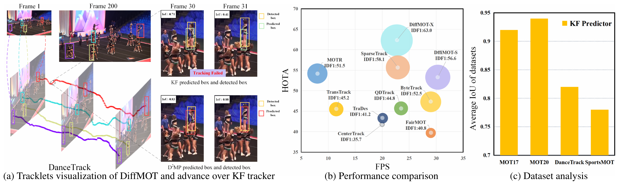
Panel (c) on the right is where this paper starts. The authors use a Kalman filter to predict the next frame's box and compute its IoU with the ground-truth box. The average IoU is above 0.9 for both MOT17 and MOT20; DanceTrack is only about 0.82, SportsMOT about 0.78.
For tracking, when predicted boxes don't line up, association has to lean on other cues to hold together. Switch to a neural network for prediction, and simple networks like MLPs and LSTMs can't fit such complex motion; methods that use optical flow or Transformers fit it better but are too slow for real time.
DiffMOT aims to predict nonlinear motion accurately and still run fast enough.
Solving the problem
Overall architecture
DiffMOT is a standard detect-then-associate tracker, in three steps:
- Detection. YOLOX finds all the boxes in this frame.
- Motion prediction. For each existing track, use its information from the past 5 frames to predict its position in this frame. This step is the core of DiffMOT, called D²MP (decoupled diffusion-based motion predictor).
- Association. It reuses ByteTrack's two-stage matching: high-score detection boxes are first matched to the predicted boxes using appearance and IoU, and what's left is matched once more against the low-score boxes using IoU. For appearance, it borrows Deep OC-SORT's dynamic appearance and adaptive weighting.
Apart from step two, everything is an off-the-shelf component. So the experiments in this paper can be read as swapping the Kalman filter for a diffusion model inside the same framework.
What gets generated is the "displacement"
D²MP doesn't generate boxes; it generates how a box changes. The motion at frame is defined as:
Once the motion is predicted, adding it to the previous frame's box gives this frame's predicted box.
The model learns the motion distribution of all the objects in the whole dataset, and at prediction time conditions on a single object's own history. The authors consider this more stable than fitting a separate motion model for each track: dancers' moves vary endlessly, but "how dancers move" does follow patterns.
A decoupled diffusion process
In an ordinary diffusion model, the forward process turns data into noise step by step. D²MP adopts a "decoupled diffusion" approach that splits this process into two halves running at the same time:
- Data decay. The clean motion data decays linearly with time and becomes zero at .
- Noise growth. Gaussian noise is added starting from zero and becomes pure noise at .
Adding the two together gives the noised motion:
is the rate of decay, and is standard normal noise. At it's the clean motion; at only is left.
The reverse process has to recover the motion from noise. The original decoupled diffusion needs a two-branch network that predicts and at the same time. The authors noticed that the equation above lets be expressed in terms of and , so the network only has to predict one quantity, .
More importantly, this process can be completed in one step.
How the one step works
Let's walk through the forward and reverse processes with an example.
Say a dancer's box in the previous frame is : center , center , width and height, in pixels. In this frame the dancer moves 12 to the right and 3 up, with the same size, so the true motion is .
In the forward process, . At :
The motion has decayed by a quarter and is mixed with noise at half a standard deviation. By , only is left.
In reverse, it jumps from straight to in one step. Plugging into the reverse-process formula, the mean comes out exactly equal to , with a variance of 0. If the network infers from the history, the predicted motion is and the predicted box is .
Worked example for this note.
An ordinary diffusion model runs hundreds to thousands of steps; in decoupled diffusion the decay is analytic and can be done in one step, so the time spent on motion prediction becomes negligible.
Where the condition comes from
To predict , the model relies on a network called HMINet. It reads this track's information from the past 5 frames, eight numbers per frame: the four values of the box, plus that frame's displacement.
These 5 frames, together with a learnable class token, first pass through 6 layers of multi-head self-attention, and the class token that comes out the other end is the condition embedding. Next, the noised motion and the condition embedding go together into a "motion fusion layer": the condition embedding passes through an MLP to produce a scale and a shift that adjust the features of the noised motion. After a few more layers of self-attention and fusion, a final MLP outputs .
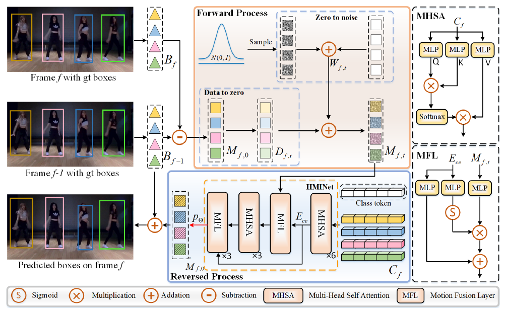
During training, the loss is the smooth L1 between the predicted and the true .
Discussion
Swapping out the motion model
The ablations are all on the DanceTrack validation set, with the detector and association unchanged and only the motion model swapped:
| Motion model | HOTA | IDF1 | AssA |
|---|---|---|---|
| IoU only | 44.7 | 36.8 | 25.3 |
| Kalman filter | 46.8 | 52.1 | 31.3 |
| LSTM | 51.2 | 51.6 | 34.3 |
| Transformer | 54.6 | 54.6 | 38.1 |
| D²MP | 55.7 | 55.2 | 39.5 |
Compiled from Table 5 of the paper, DanceTrack validation set.
The Kalman filter is only 2.1 HOTA better than no prediction at all; switching to D²MP adds another 8.9 over the Kalman filter. The Transformer isn't bad either, at HOTA 54.6, but the paper doesn't list its speed within the same framework.
Is one step enough?
| Architecture | Steps | HOTA | FPS |
|---|---|---|---|
| Two-branch | 1 | 44.5 | 20.9 |
| Two-branch | 10 | 52.3 | 13.1 |
| Two-branch | 20 | 54.6 | 7.5 |
| Single-branch | 1 | 55.7 | 22.7 |
Compiled from Table 6 of the paper, DanceTrack validation set; speed includes YOLOX-X detection.
This table shows the payoff of a single branch. The two-branch version, which predicts and together, gets only 44.5 with one sampling step and needs 20 steps to reach 54.6, by which point it's down to 7.5 FPS. The single-branch version, which predicts only , gets 55.7 in a single step. With one fewer quantity to learn, the network actually learns better.
How much history?
For the history length used as the condition, going from 1 frame to 10 frames, HOTA is 51.7, 52.5, 53.0, 55.7 (5 frames), 52.5 and 51.1 in turn. Too short, and you can't tell where the object is heading; too long, and the old information actually gets in the way of prediction. Five frames is best.
Three kinds of condition content were also tried: only the previous frame's box, only the previous frame's displacement, or both. Using both gives the highest HOTA, though the three differ by at most 1.3.
Test-set results
| Dataset | DiffMOT | Best other | Method |
|---|---|---|---|
| DanceTrack | 62.3 | 61.3 | Deep OC-SORT |
| SportsMOT | 76.2 | 74.1 | MixSort-OC |
| MOT17 | 64.5 | 65.1 | SparseTrack |
| MOT20 | 61.7 | 63.9 | Deep OC-SORT |
Test-set HOTA. DanceTrack compiled from Table 1 of the paper; SportsMOT from Table 2 of the paper, with the detector trained on the training plus validation sets; MOT17 from Table 3 of the paper; MOT20 from Table 9 in the paper's appendix.
On DanceTrack and SportsMOT, where nonlinear motion dominates, DiffMOT is first on both. On DanceTrack, its IDF1 of 63.0 and AssA of 47.2 are also 1.5 and 1.4 higher than Deep OC-SORT, so the gain is mainly in association.
On the pedestrian-heavy MOT17 and MOT20, DiffMOT is no longer the best, a little behind Deep OC-SORT and SparseTrack. Pedestrian motion is close to a straight line to begin with, the Kalman filter already does the job, and the diffusion model has little room to show what it can do.
As for speed, it runs at 22.7 FPS with YOLOX-X; switching to YOLOX-S gets it to 30.3 FPS, while HOTA drops to 53.3.
Across datasets
In the appendix, the authors take the D²MP trained on DanceTrack and apply it directly to other datasets. On SportsMOT it gets HOTA 75.6, only 0.6 below the version trained on SportsMOT, and still above MixSort-OC's 74.1. On MOT17 it's 2.7 lower.
Judging by the results, the motion of dancers and players is closer to each other than to that of pedestrians.
When it fails
The appendix lists two kinds of failure. The first is two people swapping IDs as they cross paths, which the authors attribute to the model having no constraint on the direction of velocity. The second is that people who disappear for a long time can't be recovered: D²MP only predicts one frame ahead at a time, so for a track that has been broken for a long while, it has no way of pushing forward several frames to wait for the person.
Conclusion
DiffMOT changes only one part, replacing the Kalman filter in the detect-then-associate framework with a diffusion model.
The key to making it usable for real-time tracking is decoupled diffusion. The data decay is analytic, so the reverse process can be done in one step; the network only has to predict the decay rate , which is easier to learn than predicting and the noise together. The result is a predictor that can fit the irregular motion of dancers and players and, detection included, still runs at over 20 FPS.
Compared with DiffusionTrack from half a year earlier, both papers use diffusion models: DiffusionTrack uses one to generate paired boxes for two frames, DiffMOT only to generate displacements. On DanceTrack, the latter's HOTA is higher by nearly 10.