[21.05] MLP-Mixer

Less Loss is Gain

MLP-Mixer: An all-MLP Architecture for Vision

---

After Transformers were introduced into the field of computer vision, many studies began exploring ways to make the exchange of information between patches more efficient.

Thus, a new term emerged: "Token-Mixer."

As the name implies, the purpose of a Token-Mixer is to mix information between different patches to enhance the performance of the model.

The traditional self-attention mechanism is one such implementation of a Token-Mixer.

However, due to the high computational complexity of the original attention mechanism, the academic community began searching for alternatives.

MLP-Mixer is one of these alternatives.

tip

Token-Mixer is a term coined in later papers and is not a proprietary term introduced in this paper.

Problem Definition

The authors believe: the complexity of self-attention is too high, so let's just get rid of it!

But what should we do after getting rid of it?

Hey! Look, there's a simple fully connected layer by the roadside! Let's use it!

And then the paper ends here. (Not really!)

Solution

Model Architecture

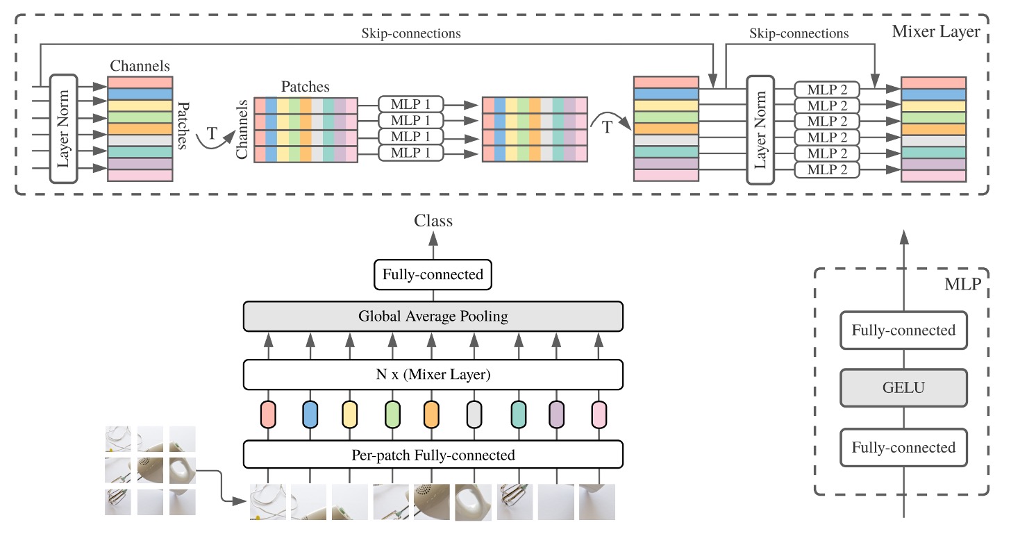
In this paper, the authors propose using two stages of fully connected layers, or MLPs (Multi-Layer Perceptrons), to exchange information.

The image above might be hard to understand, but don't worry, let's break it down step by step:

1. Input an image of size 3 x 224 x 224 and divide it into 16 x 16 patches, with a dimension assumed to be 512.

   • Dimension change: [B x 3 x 224 x 224] -> [B x 512 x 14 x 14].

2. Convert it into Transformer input format.

   • Dimension change: [B x 512 x 14 x 14] -> [B x 512 x 196].

3. First stage: Exchange information between patches.

   import torch.nn as nn
   
   patch_mixer = nn.Linear(196, 196)
   
   # Input dimension: x = [B x 512 x 196]
   x_mix_patch = patch_mixer(x)
   
   # skip connection
    x = x + x_mix_patch

4. Second stage: Exchange information between channels.

   import torch.nn as nn
   
   channel_mixer = nn.Linear(512, 512)
   
   # Input dimension: x = [B x 512 x 196]
   # Reshape first -> [B x 196 x 512]
   x_mix_channel = x.permute(0, 2, 1)
   x_mix_channel = channel_mixer(x_mix_channel)
   
   # Reshape back
   x_mix_channel = x_mix_channel.permute(0, 2, 1)
   
   # skip connection
   x = x + x_mix_channel

This completes one operation of the MLP-Mixer.

You'll notice that in the above process, the second stage is similar to the original self-attention mechanism, which also involves an MLP operation.

The difference lies in the first stage, where instead of calculating the patch self-attention map, a fully connected layer is used directly.

Discussion

Performance on ImageNet

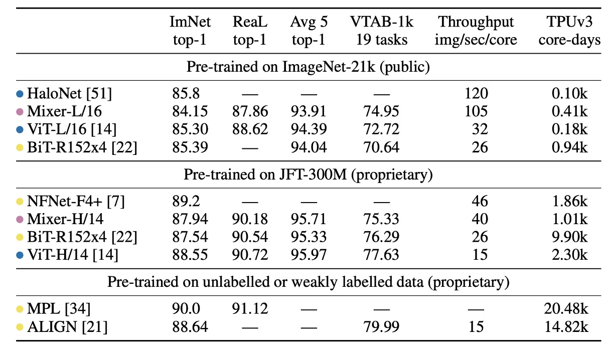
• The "ImNet" and "ReaL" columns represent the results on the original ImageNet validation set and the cleaned ReaL label set, respectively.
• Avg 5 indicates the average performance across five downstream tasks (ImageNet, CIFAR-10, CIFAR-100, Pets, Flowers).

---

When pre-trained on ImageNet-21k with additional regularization, MLP-Mixer achieves 84.15% top-1 accuracy on ImageNet. This is strong performance, but slightly below other models. Without regularization, Mixer tends to overfit, consistent with observations for ViT.

When training MLP-Mixer from scratch on ImageNet, Mixer-B/16 scores 76.4% at resolution 224, similar to a standard ResNet50 but lower than other state-of-the-art CNN/hybrid models like BotNet (84.7%) and NFNet (86.5%).

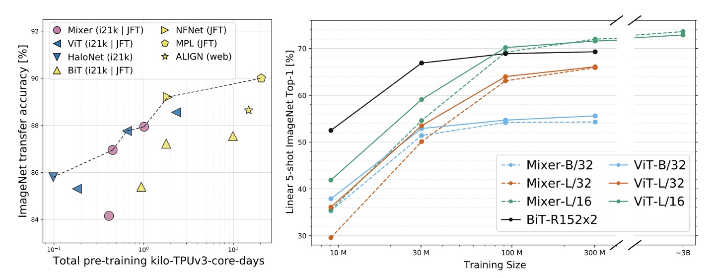
As the size of the upstream dataset increases, MLP-Mixer's performance improves significantly.

Mixer-H/14 achieves 87.94% top-1 accuracy on ImageNet, outperforming BiT-ResNet152x4 by 0.5%, but trailing ViT-H/14 by 0.5%. Mixer-H/14 runs 2.5 times faster than ViT-H/14 and nearly twice as fast as BiT.

In terms of precision-computation trade-offs, Mixer is competitive with more traditional neural network architectures. There is a clear correlation between total pre-training cost and downstream accuracy across architecture categories.

Visualization Analysis

It is generally observed that the first layer of CNNs tends to learn Gabor-like detectors, which act on local regions of the image pixels.

In contrast, MLP-Mixer allows global information exchange between tokens in the MLP, raising the question:

• Does it process information in a similar way?

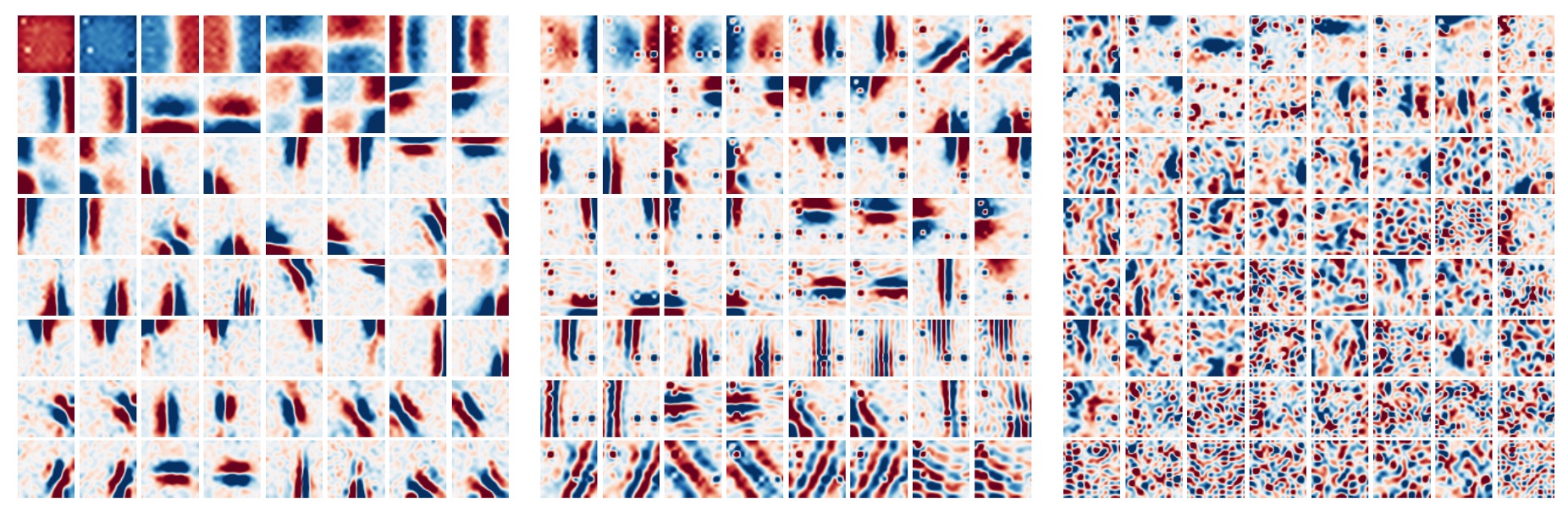
To answer this, the authors visualized features from different layers of MLP-Mixer, showing various levels of feature extraction.

In the image above, from left to right, are the first, second, and third layers of MLP-Mixer. We can see:

• Some learned features act on the entire image, while others act on smaller regions.
• Deeper layers seem to have less distinguishable structures.
• Similar to CNNs, there are many feature detectors with opposite phases.

Conclusion

Less loss is gain!

Compared to the original self-attention mechanism, MLP-Mixer significantly reduces computational complexity. Even if the performance is slightly worse, it still has a strong market appeal!