[20.02] SimCLR v1

Z. Yuan

Dosaid maintainer, Full-Stack AI Engineer

Winning with Batch Size

A Simple Framework for Contrastive Learning of Visual Representations

---

Contrastive learning has been researched for about five years, and the entire field has become highly complex and chaotic. Not only are architecture designs intricate, but the specific model training methods are also varied.

The authors of this paper believe that the core of contrastive learning should be simpler.

Defining the Problem

Recall the essential elements of contrastive learning:

• To achieve good results, is a memory bank really necessary?

We need a large number of negative samples to guide the model in learning better representations, and a memory bank can indeed serve this purpose. The original InstDict did this, and later MoCo followed suit.

But it's annoying! Maintaining a memory bank during training is clearly an unfriendly design.

In this paper, the author decides to directly discard the memory bank design, opting for larger batch sizes instead. As long as we provide enough negative samples, the model can learn sufficiently good representations!

tip

For readers who haven't read InstDict or MoCo, you can refer to our previous articles:

• [18.05] InstDisc: More is Better
• [19.11] MoCo v1: Momentum Contrastive Learning

Solving the Problem

Model Architecture

This architecture is really simple: no multiple encoders, no memory bank.

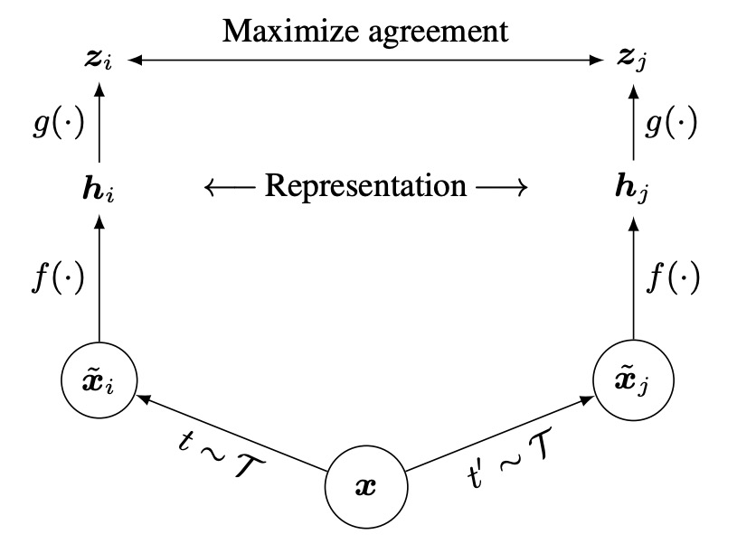
The process starts by applying two random augmentations to the same image, producing two "seemingly different, but actually from the same source" images.

Then, both images are passed through "the same" encoder network to obtain two latent vectors.

Next, a small projection network maps these latent vectors to the contrastive learning space, and finally, a contrastive loss function ensures that the "same source" augmented images are close to each other in the representation space.

Huh? That's it?

Yes! That's it, and we've just finished reading a paper! (Not really)

Image Augmentations

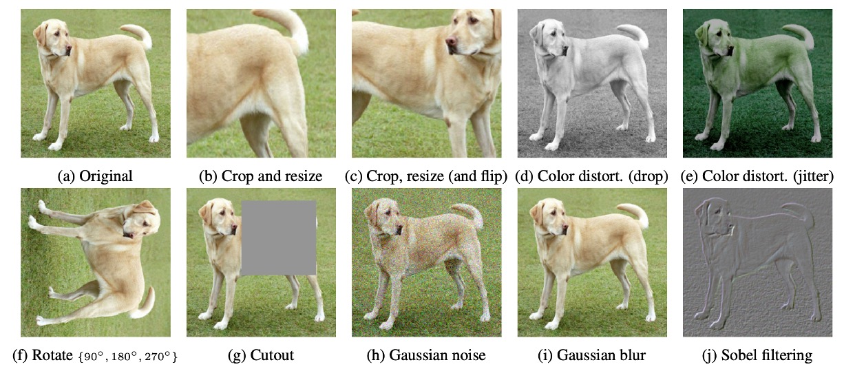
In SimCLR, the authors believe that augmentations are diverse and powerful, more important than supervised learning.

The augmentations used in the paper are shown in the figure above, and the key ones include:

• Random crop
• Color distortion
• Gaussian blur

The two augmented images are treated as a "positive pair" because they both come from the same original image.

Detailed Design

First, for the encoder, ResNet-50 is used as the base encoder. The augmented images are input into the network to obtain a vector $h_i$. The dimensionality of this vector is typically large, such as 2048 dimensions after average pooling for ResNet-50.

Next, for the projection head, the authors found that applying the contrastive loss directly on $h_i$ is less effective than adding a small MLP first. This projection network $g(·)$ typically consists of one hidden layer, followed by ReLU, and then projecting onto a 128-dimensional vector $z_i$ used for contrastive loss calculation.

The most critical part is how to define the contrastive loss.

The core concept is: for the same pair $(i, j)$ (which come from the same original image), they should be as close as possible in the vector space, while being as far apart as possible from unrelated samples. Here, the authors refer to the NT-Xent (Normalized Temperature-scaled Cross Entropy Loss) formulation.

NT-Xent Loss Function

This is essentially the InfoNCE loss function we have seen before, except that the authors have modified the input format while keeping the formula unchanged. Here, ℓ₂ normalization is applied to the input features, which stabilizes the calculation of cosine similarity.

tip

If you are interested in the paper that introduced InfoNCE, you can refer to:

• [18.07] CPC: Today shapes tomorrow

The NT-Xent loss function is computed as follows:

$$ℓ_{i,j} = - \log \left( \frac{\exp(\text{sim}(z_i, z_j)/τ)}{\sum_{k=1}^{2N} \mathbf{1}[k \neq i] \exp(\text{sim}(z_i, z_k)/τ)} \right).$$

Where:

• $zᵢ$ is the 128-dimensional vector obtained from the projection head after processing the $i$-th augmented image.
• $\text{sim}(u, v) = \frac{u^\top v}{\|u\|\|v\|}$ represents cosine similarity.
• $τ$ (tau) is the temperature hyperparameter, which controls the scaling of similarity scores.
• The numerator, $\exp(\text{sim}(z_i, z_j)/τ)$, represents the exponentiated similarity score between $z_i$ and the positive sample $z_j$.
• The denominator is the sum of the exponentiated similarity scores between $z_i$ and all other vectors in the batch (excluding itself).

In a batch, assume there are $N$ original images, each undergoing two different augmentations, resulting in a total of $2N$ augmented images. For a positive pair $(i, j)$ (i.e., two different augmentations of the same original image), the loss is computed while treating the remaining $2(N - 1)$ augmented images as negative samples.

The objective is to maximize the similarity between positive samples $(z_i, z_j)$ while minimizing the similarity of all other negative samples. That is, we aim for $\text{sim}(z_i, z_j)$ to be much greater than $\text{sim}(z_i, z_k)$ (for all $k \neq i$). This encourages the model to learn more discriminative representations, ensuring that similar samples cluster together while dissimilar samples are pushed apart.

Within a batch, for each positive pair $(i, j)$, both $(i, j)$ and $(j, i)$ losses are computed and summed for backpropagation.

tip

NT-Xent adapts the impact of negative samples using cosine similarity (with ℓ₂ normalization) and the temperature parameter ($\tau$).

• Cosine similarity: Ensures the model focuses on the direction of vectors rather than their magnitude, leading to a more accurate comparison of relative similarities.
• Temperature parameter ($\tau$): Controls the scaling of similarity scores, affecting the weighting of negative samples in the loss function:
  • Small $\tau$ → Enlarges similarity differences → Emphasizes hard negatives.
  • Large $\tau$ → Smooths similarity differences → Negative samples have a more balanced impact.

In traditional contrastive loss functions, to properly handle the impact of easy/hard negative samples, manual semi-hard negative mining is often required. Without this selection, most negative samples may be too easily distinguishable (leading to excessive contrast), which could reduce the effectiveness of learning.

However, NT-Xent dynamically adjusts the weighting of negative samples based on similarity scores using cosine similarity + temperature scaling, eliminating the need for manual negative sample selection. Experiments have shown that contrastive loss functions like logistic loss and margin loss generally perform worse without semi-hard negative mining. Even when semi-hard negative mining is applied, they may still not outperform NT-Xent.

Discussion

Most Useful Augmentation Combinations

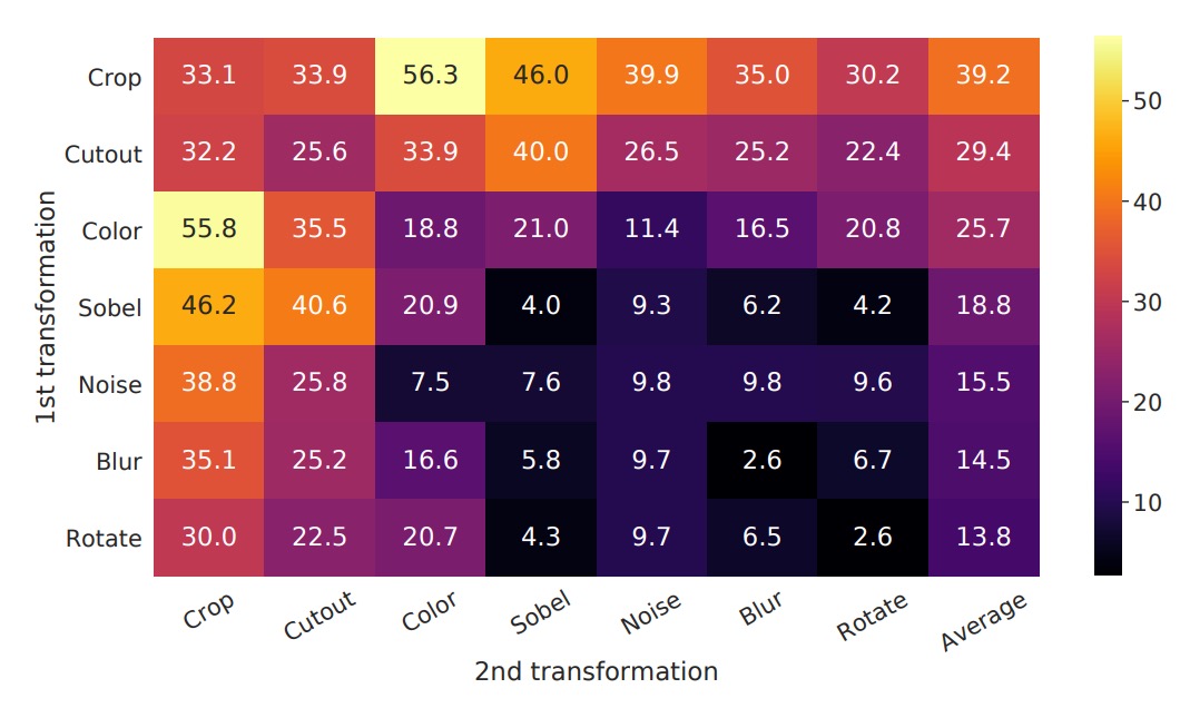
To observe the impact of different data augmentation methods (either individually or in combination) on the quality of representations learned by the model, the authors use linear evaluation. In this approach, the pre-trained encoder is frozen, and a linear classifier (usually a fully connected layer) is added on top, followed by top-1 accuracy evaluation on ImageNet.

In the experiment, the model input has two "parallel augmentation pipelines." Here, the authors intentionally apply the tested augmentation to "one of the pipelines," while the other branch applies only basic random crop + resize. This allows a clearer observation of the effects of individual augmentations or combinations, without their effects being mixed.

The interpretation of the table in the image is as follows:

• Diagonal entries: Single transformations (e.g., Gaussian blur, color distortion), representing the application of only that augmentation to one branch.
• Off-diagonal entries: Combinations of two augmentations (e.g., first Gaussian blur, then color distortion).
• Last column: The average value of each row, which is the average performance under the augmentation combination for that row.

The experimental results show:

• Single augmentations (diagonal entries) are usually not enough for the model to learn strong representations. With only one variation, the model can still rely on other invariant cues to identify "positive pairs."
• Augmentation combinations (off-diagonal entries) tend to improve linear evaluation results.

This suggests that when two or more augmentations occur simultaneously, the contrastive learning task becomes harder, but it also enables the model to learn more general and stable features.

Impact of Augmentation Strength

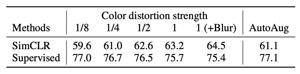
We can adjust the strength of augmentations, such as increasing or decreasing the variation in brightness, contrast, saturation, and hue. The authors further explore the impact of "augmentation strength" on model performance.

When training supervised classification models on ImageNet, auto-augmentation strategies like AutoAugment are commonly used. However, the authors find that AutoAugment is not necessarily better than the "simple crop + strong color distortion" approach.

The results, as shown in the table above, reveal that for unsupervised contrastive learning, increasing the strength of color distortion significantly improves the quality of features learned by the model. This indicates that the required augmentations for unsupervised contrastive learning differ from those in supervised learning. Many augmentations that are "very effective" in supervised learning may not similarly enhance contrastive learning.

tip

For different learning goals, the choice of augmentation strategy may differ. However, we often subconsciously overlook this issue because other factors might seem more important.

The author's experimental results remind us that the selection of augmentation strategies can have a significant impact on model learning effectiveness, making it worthwhile to carefully tune this aspect.

Scaling Up the Model

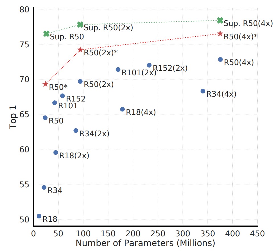
The figure above shows the performance of contrastive learning at different model scales. The authors find that as the model size increases, the performance of contrastive learning improves progressively.

This result is similar to our experience in supervised learning: increasing model capacity typically allows for richer feature representations. Additionally, as model size increases, the improvement in unsupervised contrastive learning becomes more evident, suggesting that contrastive learning is even more dependent on large models than supervised learning.

tip

Why does unsupervised learning perform worse with small models compared to supervised learning, but can compete when models are large?

In unsupervised settings, the model needs to discover the data structure on its own. If the model is too small, its representational space is highly constrained, preventing it from learning sufficiently rich features. However, once the model capacity is large enough, it can capture a variety of patterns that are observable without labels, which might be even richer than the labels used in supervised learning.

Batch Size Impact

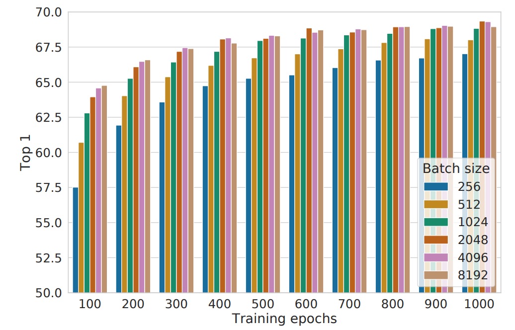
The figure above shows performance at different batch sizes and training durations, with each bar representing the result from a single training experiment.

Traditionally, batch size selection mainly considers computational efficiency and gradient stability. However, in contrastive learning, batch size also plays a crucial role: it impacts the number of available negative samples.

• Larger batch sizes mean more negative samples available per training step, allowing the model to learn richer contrastive information and improve sample discrimination.
• Faster convergence: With fewer training epochs, larger batches allow the model to observe more negative samples in a shorter time, accelerating convergence and improving final performance.

This differs from supervised learning. In supervised learning, large batches mainly aim to "stabilize gradient estimates and improve training efficiency." But in contrastive learning, more negative samples are the core advantage brought by large batches.

Another interesting finding is that longer training times can partially offset the disadvantages of small batches:

• When training steps are sufficient, even small batches can accumulate enough negative sample exposure over time, narrowing the performance gap with large batches.
• However, under the same training time, larger batches typically achieve similar results faster, making them a more efficient strategy when computational resources are limited.

Comparison with Other Methods

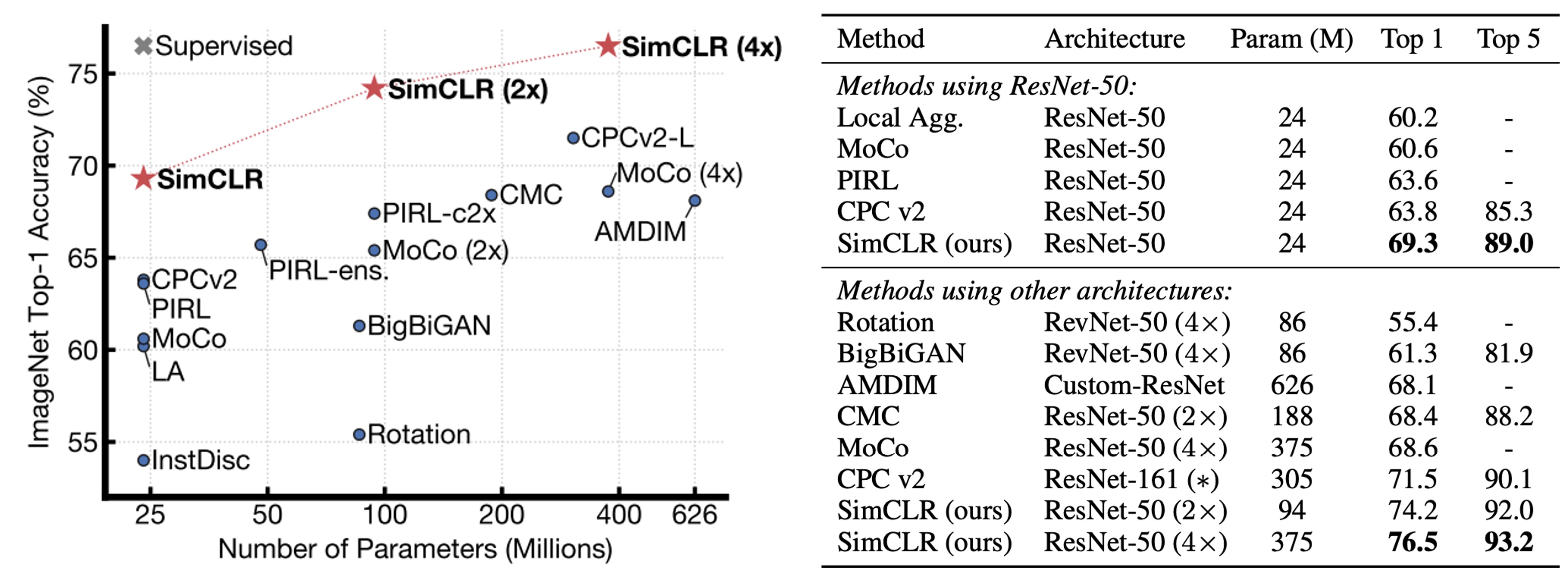
The authors compare the linear evaluation results of various self-supervised learning methods (i.e., freezing the backbone and adding a linear classifier on top).

The results show that even with the standard ResNet architecture (without special network designs), SimCLR achieves or exceeds the performance of previous methods that required specially designed network structures. When ResNet-50 is scaled up by 4×, its linear evaluation results can rival a supervised pre-trained ResNet-50, indicating that unsupervised contrastive learning has immense potential in large models.

If the number of ImageNet labels is reduced to 1% or 10%, and fine-tuning is done using class-balancing, as shown in the table below:

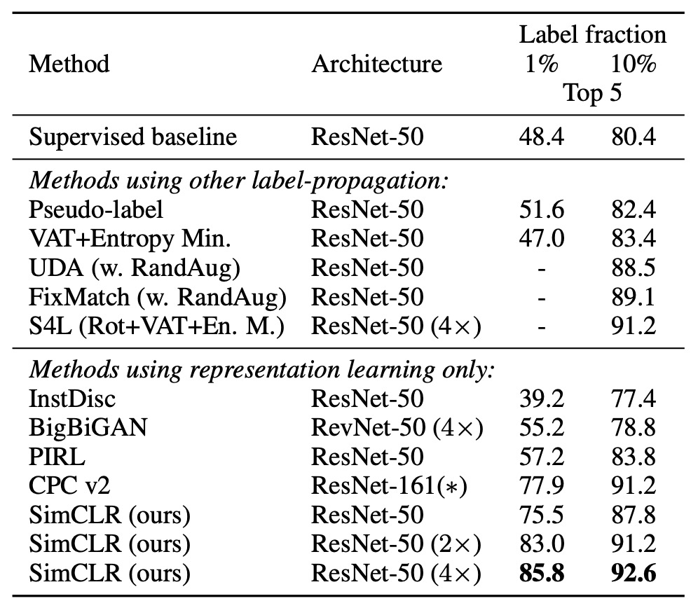
We can see that SimCLR still outperforms other methods, showing that contrastive learning has substantial potential in semi-supervised learning as well.

Conclusion

In this study, the authors propose a simple yet effective contrastive learning framework and thoroughly analyze the impact of various design choices on learning outcomes.

The results show that through data augmentation strategies, nonlinear projection heads, and the NT-Xent loss function, SimCLR significantly outperforms previous techniques in self-supervised learning, semi-supervised learning, and transfer learning tasks.

tip

Contrastive learning, with SimCLR and MoCo as the watershed, has ended the period of chaos in this field, established a clear research direction, and provided important reference points for future research.